Financial Wealth, Investment and Sentiment in a Bayesian DSGE Model
←
→
Page content transcription
If your browser does not render page correctly, please read the page content below
Financial Wealth, Investment and Sentiment in a
               Bayesian DSGE Model

                     Tao Jin∗           Simon Kwok†               Xin Zheng‡

                                             Abstract
      This paper is a quantitatively oriented theoretical study into interactions among
      macroeconomic fluctuations, stock price dynamics and investor sentiment varia-
      tions, with a focus on two episodes, namely, the 2008 Great Financial Crisis and
      the 2020 COVID-19 Pandemic. Our objectives are fivefold, namely, household
      turnover and firm turnover mechanisms are introduced to capture financial wealth
      effect and capital reallocation effect respectively, variable capital utilization and in-
      vestment shocks are incorporated to study the interplay between the stock market
      and the production sector, the labor intensity shock is specified to examine im-
      pacts of pandemics on labor intensity, and stock price fluctuations induced by the
      financial shock are disentangled from those triggered by the sentiment shock, fiscal
      and monetary policies are evaluated to examine responses to financial instability
      and coronavirus recession. We formulate a Bayesian Dynamic Stochastic General
      Equilibrium (DSGE) model for the U.S. economy, our methodologies include Chib
      and Ramamurthy (2010)’s TaRB-MH algorithm, impulse response analysis, forecast
      error variance decomposition and Bayesian model comparison. Our findings con-
      tribute to the literature along four dimensions. Household turnovers, firm turnovers,
      preference, investment and sentiment jointly influence financial wealth distribu-
      tion and financial resource allocation, inducing subsequent stock price swings and
      macroeconomic fluctuations. These are not only due to households’ interactions
      with the stock market through financial wealth and consumption, but also trig-
      gered by firms’ interactions with the stock market through financial resources and
      investment. Higher household turnover rate increases financial wealth effect and
      aggregate demand, whereas higher firm turnover rate enhances capital reallocation
      effect at the cost of contaminating financial wealth effect. Monetary policy responds
      counteractively and significantly to financial slack at business cycle frequencies.

      Keywords
      Financial wealth effect;     Capital reallocation effect;    Labor intensity shock;
  ∗
     PBC School of Finance, Tsinghua University. Jin is supported by the National Natural Science
Foundation of China (Project No.’s: 71828301 and 71673166).
   †
     School of Economics, the University of Sydney.
   ‡
     Corresponding Author. Research Center for Finance Development, PBC School of Finance, Tsinghua
University and School of Economics, the University of Sydney. Email: zhengx@pbcsf.tsinghua.edu.cn.
Zheng is supported by University of Sydney International Scholarship, China International Exchange
Fellowship and Tsinghua Postdoctoral Fellowship.

                                                 1
Variable capital utilization   Sentiment       Stock market bubble   TaRB-MH

     JEL Classification
     E44; E52; C51

1.    Introduction
History has not only witnessed financial markets’ function in signaling economic uncer-
tainty and financial fragility, but also revealed the growing dependence between financial
variability and macroeconomic fluctuations. For instance, the 2008 Great Financial Crisis
sparked the 2009 Great Recession, whereas the 2020 COVID-19 Pandemic triggered the
2020 Stock Market Crash and the Deep Recession. Consequently, it is crucial to under-
stand mechanisms through which stock price fluctuations propagate to the real economy,
channels through which macroeconomic aggregates influence stock price swings, and mon-
etary policy rules through which central banks respond to financial instability. These shed
light on prevention of financial crises’ propagation to the real economy, mitigation of eco-
nomic uncertainties’ impacts on financial markets, and development of monetary policy
tools to ensure financial stability.
    The literature has mainly investigated demand-side interaction between stock price
fluctuations and the real economy in the Dynamic Stochastic General Equilibrium (DSGE)
framework. Castelnuovo et al. (2010), Funke et al. (2011), and Nisticò (2012) introduce
the household turnover mechanism and examine financial wealth effect through demand-
side of the real economy. They not only find that stock prices are essential in influencing
real activities and driving business cycles, but also identify significant and counterac-
tive responses of central banks to stock price misalignments. However, they incorporate
neither the firm turnover mechanism nor physical capital accumulation, neglecting the
stock market’s influence through supply-side of the real economy, Furthermore, their
models do not account for frictions in utilizing labor capacity and therefore cannot cap-
ture pandemics’ impacts upon production through labor intensity. On one hand, we
include household turnover and firm turnover mechanisms to capture macroeconomic con-
sequences of financial wealth and capital reallocation effects respectively. On the other
hand, we specify the labor intensity shock and incorporate capital capacity utilization
data, with the purpose of studying impacts of pandemics on macroconomic fluctuations.
From the demand-side, stock price fluctuations, which reflect household expectations
about future wealth, influence household intertemporal substitution of consumption and
decisions through household financial wealth. Specifically, incumbent household traders
with financial wealth incur a probability of exiting financial markets and being replaced
by new traders without financial wealth, their financial wealth is redistributed among
surviving households. Incumbent household traders use accumulated financial wealth
to smooth consumption, whereas new traders without financial wealth cannot smooth
consumption. Nonetheless, individual consumption smoothing does not imply the same
level of aggregate consumption smoothing. Therefore, when household turnover rate
increases, the difference between current and expected future average consumption is
greater. These influence stochastic discount factor and subsequently affect household

                                                2
behavior. In consistence with Castelnuovo et al. (2010)’s analysis, we find increases in
household financial wealth convey higher purchasing power, creating a financial wealth
effect. From the supply-side, stock price swings, which signal expectation about future
market capitalization, influence wholesale firms’ investment, production and dividends
through credit constraints, physical capital accumulation and firm budgets respectively.
Concretely, when firm turnover rate γW increases, more new wholesale firms replace
incumbent wholesale firms, and new wholesale firms are more likely to contain stock
bubbles than incumbent wholesale firms, consequently, more stock bubbles lessen credit
constraints and generate more financial resources for new wholesale firms. Higher firm
turnover rate amplifies capital reallocation effect, leading investment to more productive
wholesale firms. Since investment may crowd out consumption, capital reallocation effect
contaminates financial wealth effect, and larger financial wealth effect is associated with
lower firm turnover rate.
Castelnuovo et al. (2010), Funke et al. (2011), Nisticò (2012), and Miao et al. (2015)
elucidate macroeconomic consequences of stock price swings under the assumption that
central banks target at zero inflation, although zero inflation targeting is rare in the real
economy. However, in our model, central banks use a positive inflation target in the
monetary policy rule, and a proportion of wholesale firms update prices according to
past inflation and the positive inflation target.
Furthermore, along the lines of Castelnuovo et al. (2010), Funke et al. (2011) and
Nisticò (2012), in order to investigate the interplay between the stock market and the
production sector, we not only specify our DSGE model with variable capital utilization,
physical capital accumulation and credit constraints, but also buffet our DSGE model
with the labor intensity shock, the marginal efficiency of investment shock, the idiosyn-
cratic investment shock, the financial shock and the sentiment shock. On one hand,
these specifications provide channles through which pandemics influence labor intensity,
capital utilization, market capitalization and financial slackness in the production sector,
as well fluctuations in the stock market. On the other hand, these shocks capture im-
pacts of stock market uncertainty upon investment efficiency, financial flexibility, dividend
prospects and investor expectation in the producton sector.
Last but not least, the DSGE models of Castelnuovo et al. (2010), Funke et al. (2011),
and Nisticò (2012) do not explicitly distinguish between stock price misalignments ex-
plained by macroeconomic fundamentals and stock price fluctuations induced by investor
sentiment. Our DSGE model, however, elucidates that forces driving episodes of stock
market booms and busts encapsulate both economic fundamentals and sentiment. On
one hand, economic fundamentals explain procyclicality of stock market indices. On the
other hand, sentiment not only drives evolution of speculative stock bubbles and fluctu-
ations of stock prices, but also influence the real economy through credit constraints and
investment. Castelnuovo et al. (2010) do not disentangle the effect of the financial shock
from that of the sentiment shock. However, we decompose stock price into fundamental
value perturbed by the financial shock and speculative bubble driven by the sentiment
shock. The financial shock captures financial frictions in firms’ new equity issuance,
limited loan contract enforceability and collateral constraints. We not only formulate a
microfoundation for speculative stock bubbles to enter the stock market, but also replace
3Castelnuovo et al. (2010)’s stock market index measurement error with the sentiment
shock. The sentiment shock reflects proportional size change between old and new spec-
ulative stock bubbles, particularly agents’ optimistic or pessimistic beliefs about future
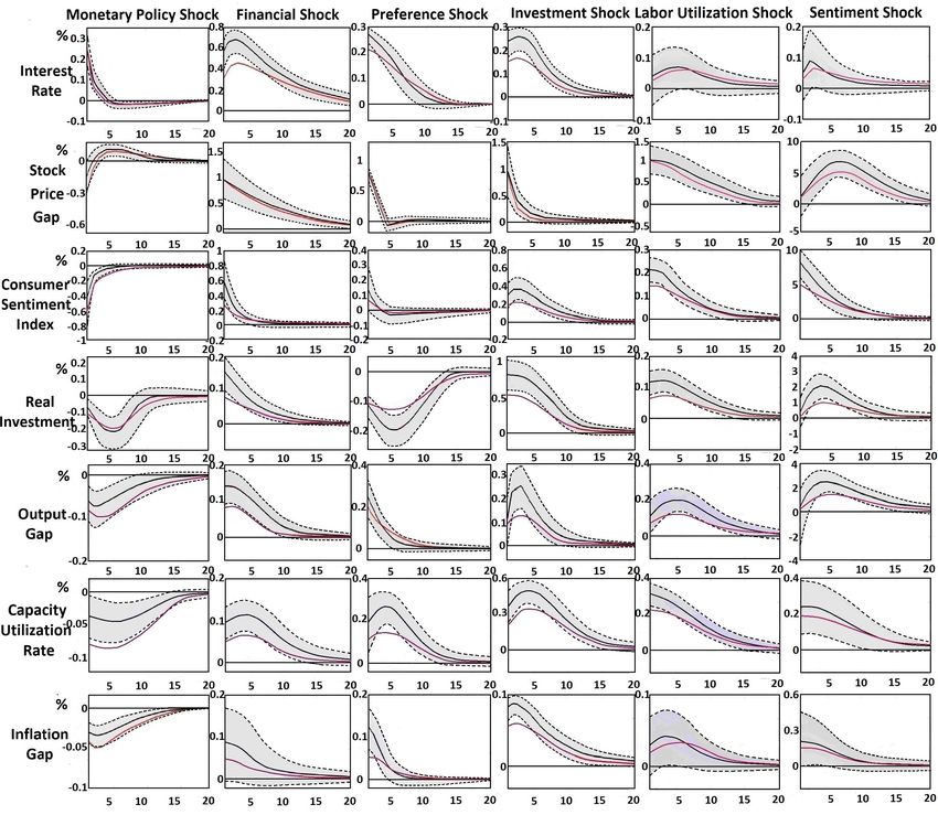
stock market. According to impulse response analysis and forecast error variance decom-
position, we find both the financial shock and the sentiment shock play essential roles in
triggering financial crisis and magnifying economic recessions. In consistence with Miao
et al. (2015)’s analysis, we find rises in stock bubbles signal more firm budget flexibility
and higher investment profitability. Therefore, financial resources move to more prof-
itable and efficient firms, strengthening capital reallocation effect. Excess stock market
fluctuations and asset price misalignments contradict central banks’ goal of financial sta-
bility. Therefore, central banks generally respond to stock price misalignments through
monetary policy rules.
The remaining of this paper is organized as follows. Section 2 specifies the model
structure. Section 3 summarizes the data, performs estimation and conducts model
comparison. Section 4 elucidates the model dynamics. Section 5 concludes the paper.
2. The Baseline DSGE Model
The economy consists of households, capital good firms, final good firms, retail firms,
wholesale firms, financial intermediaries, the central bank and the government. House-
holds supply labor to wholesale firms, deposit at financial intermediaries, purchase gov-
ernment bonds, pay taxes to the government, purchase final goods from final good firms,
and trade stocks in the stock market. Capital good firms transform final goods purchased
from final good firms into investment goods, and sell investment goods to wholesale firms.
Wholesale firms borrow from financial intermediaries, issue stocks to households, em-
ploy labor from households, purchase investment goods from capital good firms, combine
investment goods with undepreciated physical capital to accumulate installed physical
capital, produce and sell wholesale goods to retail firms. Retail firms transform homoge-
neous wholesale goods into heterogeneous retail goods, and sell retail goods to final good
firms. Final good firms assemble retail goods purchased from retail firms to produce
final goods, and sell final goods to households, capital good firms and the government.
Financial intermediaries not only absorb deposits from households and wholesale firms
with non-binding credit constraints, but also issue corporate loans to wholesale firms with
binding credit constraints. The government imposes taxes on households and issues gov-
ernment bonds to finance government spending. The central bank adjusts interest rate
in response to inflation gap, output gap and financial slack. Nominal variables, which
include final good prices and retail prices, are denominated in currency.
2.1. Households
We model household behavior along the lines of Castelnuovo et al. (2010), Funke et
al. (2011) and Nisticò (2012). In period 0, the household sector is populated by a unit
continuum of cohorts of households, and i-period-old households are categorized into
cohort i, because they enter economic life at age i. Although households are heterogeneous
4in terms of the ages that they enter financial markets, households belonging to the same
cohort are homogeneous, and the aggregate behavior of each cohort is modelled by the
decision-making process of the representative household within each cohort. Assuming no
population growth, from period 1 onwards, incumbent household traders incur a constant
probability γH of dying, exiting financial markets and being replaced by a commensurate
fraction of new household traders without financial wealth. Since cohort size is1 γH , its
implied effective economic decision horizon is2 γ1H . Both incumbent and new household
traders purchase consumption goods from final good firms, supply labor to wholesale
firms and pay taxes to the government. However, only incumbent household traders hold
financial assets.
2.1.1. Human Wealth
Since household traders affiliated with cohort i are endowed with labor, own capital
good firms and retail firms, they obtain wages from supplying labor [Ht (i)] to whole-
sale firms, as well as gaining profits from capital good firms and retail firms. At the
beginning of each period, cohort i possesses nominal human wealth [PY,t HWt (i)], which
is the present discounted value of cohort i’s future cash inflows generated by labor wages
R1
[PY,t+ι Wt+ι νH,t+ι Ht+ι (i)], wholesale firms’ profits [ 0 ΓY,t+ι (l)dl] and capital good firms’
profits [PY,t+ι ΓK,t+ι (i)], net of cash outflows induced by lump-sum taxes [PY,t+ι Tt+ι (i)].
Concretely, human wealth originating from labor endowment and firm ownership are the
present discounted values of nominal wages and nominal profits respectively accruing in
the future to cohorts currently alive. Assuming cohorts exhibit homogeneity in labor pro-
ductivity and firm ownership, wage income, profits and taxes are all uniformly distributed
across cohorts so that they are independent of cohort age i.
+∞
X Z 1
ι
PY,t HWt (i) = Et ηt,t+ι (1 − γH ) PY,t+ι [Wt+ι νH,t+ι Ht+ι + ΓY,t+ι (l)dl + ΓK,t+ι − Tt+ι ]
ι=0 0
(1)
where ηt,t+ι is equilibrium nominal stochastic discount factor. (1 − γH ) is household
survival probability in each period and captures uncertain economic life span.
2.1.2. Financial Wealth
Households of cohort i begin trading in financial markets at the age of i. Specifically,
incumbent households not only obtain payments from government bond holdings and
deposit holdings, but also receive dividends from stock holdings. At the beginning of each
period, cohort i obtains bond wealth [BWt (i)] from holding government bonds [Bt (i)]:
PY,t BWt (i) = PY,t Bt (i) (2)
gains deposit wealth [DWt (i)] from holding deposits [DEt (i)] in financial intermediaries:
PY,t DWt (i) = PY,t DEt (i) (3)
1
Pt Pt
In period t, aggregate household population= i=−∞ γH (1 − γH )t−i = γH i=−∞ (1 − γH )t−i = 1,
where γH is cohort i’s size, and (1 − γH )t−i is cohort i’s accumulated survival probability to period t.
P+∞
2
In period 0, cohort i’s effective economic decision horizon= t=0 (1 − γH )t = γ1H .
5R1 R1
and receives aggregate dividend [ 0 Dt (j)dj] from holding stocks [ 0 St (i, j)dj] issued by
wholesale firms survived. Concretely speaking, cohort i’s nominal stock wealth [PY,t SWt (i)]
R1
includes aggregate ex-dividend stock value [ 0 PY,t P st (j)St (i, j)dj] and aggregate divi-
R1
dend [ 0 PY,t Dt (j)St (i, j)dj]:
Z 1
PY,t SWt (i) = PY,t [P st (j) + Dt (j)]St (i, j)dj (4)
0
2.1.3. Budget Constraints and Borrowing Constraints
For cohorts of incumbent household traders in financial markets, their intertemporal bud-
get constraints require that nominal expenditure is funded by nominal income. House-
hold traders purchase financial assets at the end of period t. On one hand, nominal
expenditure includes consumption of final goods [PY,t Ct (i)], payment of taxes (PY,t Tt ),
bank deposits [PY,t+1 DEt+1 (i)], purchase of government bonds [Bt+1 (i)] and aggregate
R1
stock [ 0 PY,t P st (j)St+1 (i, j)dj]. On the other hand, nominal income includes wages
R1
[PY,t Wt νH,t Ht (i)], retail firms’ profits [PY,t 0 ΓY,t (l)dl], capital good firms’ profits (PY,t ΓK,t ),
bond wealth [PY,t BWt (i)], deposit wealth [PY,t DWt (i)] and stock wealth [PY,t SWt (i)]. Due
to the unconnectedness between incumbent and new household traders, cohorts have no
bequest motive, triggering private insurance firms to offer insurance risklessly. Specif-
ically, in period t, cohort i receives a proportionate financial wealth3 [γH F Wt (i)] from
insurance firms conditional on survival, but pays the whole financial wealth [F Wt (i)]
to insurance firms conditional on death. Therefore, the reciprocal of household sur-
1
vival probability 1−γ H
represents the insurance contract’s gross yield, and this gross yield
originates from redistributing financial wealth of households who exit financial markets
among households who remain in financial markets within the same cohort. Wholesale
firm exit probability γM influences capital reallocation effect, because higher wholesale
firm turnover indicates more new wholesale firms with stock bubbles replace incumbent
wholesale firms, inducing capital movement to more efficient firms and strengthening cap-
ital reallocation effect. Since households have no bequest motive, cohort i consumes all
resources and household budget constraint is binding in each period. Inspired by Kocher-
lakota (2009), the existence of stock bubbles requires incumbent cohort i is subject to a
borrowing constraint by holding a non-negative bank deposit [DEt+1 (i) ≥ 0].
Z 1
PY,t Ct (i) + PY,t [P st (j) + Dt (j)]St+1 (i, j)dj + Et [ηt,t+1 PY,t+1 Bt+1 (i)]
0
Z 1
1
+ Et [PY,t+1 DEt+1 (i)] + PY,t Tt ≤ PY,t Wt νH,t Ht (i) + PY,t ΓY,t (l)dl+ (5)
RD,t 0
1 1 1 − γW
PY,t ΓK,t + PY,t BWt (i) + PY,t DWt (i) + PY,t SWt (i)
1 − γH 1 − γH 1 − γH
For cohorts of new household traders in financial markets, their budget constraints
require the sum of nominal consumption [PY,t Ct (i)] and tax (PY,t Tt ) equals the sum of
3
Financial wealth [F Wt (i)] includes bond wealth [BWt (i)], deposit wealth [DWt (i)] and (1 − γW ) pro-
portion of stock wealth [SWt (i)]
6R1
nominal wages [PY,t Wt νH,t Ht (i)], retail firms’ profits [PY,t 0 ΓY,t (l)dl] and capital good
firms’ profits (PY,t ΓK,t ):
Z 1
PY,t Ct (i) + PY,t Tt = PY,t Wt νH,t Ht (i) + PY,t ΓY,t (l)dl + PY,t ΓK,t (6)
0
2.1.4. Utility Maximization
Since households derive utility from consumption of final goods but suffer disutility from
supplying labor to wholesale firms, cohort i’s additively separable utility function is in-
creasing and concave in real consumption [Ct (i)], but is decreasing and convex in effective
labor supply [νH,t Ht (i)]. The logarithmic utility specification ensures the existence of a
balanced-growth path. The intertemporal preference shock (νP,t ) influences periodical
utility through exhibiting intertemporal effects upon two adjacent periods’ utilities. The
labor intensity shock (νH,t ) perturbs household utility through leisure and accounts for
loss of working hours during unexpected public health events. In period 0, the represen-
tative household trader of cohort i chooses optimal sequences of real consumption [Ct (i)],
labor supply [Ht (i)], deposit holdings [DEt+1 (i)], government bond holdings [Bt+1 (i)] and
R1
stock holdings [ 0 St+1 (i, j)dj] to maximize the expected lifetime utility [U0 (i)], taking
into consideration that cohort i survives to period t with probability (1 − γH )t :
+∞
X
U0 (i) = E0 β t (1 − γH )t νP,t {lnCt (i) + %ln[1 − νH,t Ht (i)]} (7)
t=0
subject to a sequence of cohort i’s intertemporal budget constraints in equation (5) and
borrowing constraint of non-negative deposits4 [DEt+1 (i) ≥ 0]. where β is the intertempo-
ral discount factor and captures consumption impatience. % ∈ (0, +∞) is leisure weight.
The intertemporal preference shock (νP,t ) follows an autoregressive of order one pro-
cess in logs with an independently, identically and normally distributed preference inno-
vation (εP,t ), whose mean is 0 and standard deviation is σP :
lnνP,t = lnνP + ρP (lnνP,t−1 − lnνP ) + εP,t
(8)
εP,t ∼ i.i.d.N 0, σP2
where ρP ∈ (0, 1) is autoregressive parameter and νP is steady-state preference shock.
The labor intensity shock captures unexpected public health events’ impacts on labor
intensity, for instance, the recent COVID-19 epidemic, which is represented by a labor
intensity shock with size less than one, makes it unsafe for households to work if their
jobs require close interaction with people, and these households stay at home either by
choice or by government containment policies. The labor intensity shock (νH,t ) follows an
autoregressive of order one process in logs with an independently, identically and normally
distributed labor intensity innovation (εH,t ), whose mean is 0 and standard deviation is
σH :
lnνH,t = lnνH + ρH (lnνH,t−1 − lnνH ) + εH,t
2
(9)
εH,t ∼ i.i.d.N 0, σH
4
Since cohort i has no collateralized assets, it can neither borrow nor issue stocks.
7where ρH ∈ (0, 1) is autoregressive parameter and νH is steady-state labor intensity shock.
Household utility maximization leads to the first order conditions in Appendix A.
Intratemporal condition between real consumption [Ct (i)] and labor [Ht (i)] indicates
%ν
that the ratio of marginal utility of leisure [ 1−νH,tH,t
Ht (i)
] to marginal utility of consumption
[ Ct1(i) ] equals the ratio of nominal wage (PY,t Wt ) to nominal final good price (PY,t ):
Ct (i)%νH,t
= Wt (10)
1 − νH,t Ht (i)
where Wt is real wage, % is leisure weight.
Intertemporal conditions of consumption [Ct (i)] and government bond holdings [Bt+1,τ +1 (i)]
define equilibrium nominal stochastic discount factor (ηt,t+1 ), which discounts future
4Ct (i) MU (i)
nominal payoffs, as intertemporal substitution in consumption [ 4C t+1 (i)
= M UC,t+1 ] dis-
C,t (i)
PY,t+1
counted by intertemporal discount factor β and adjusted by future inflation πt,t+1 = PY,t :
βνP,t+1 M UC,t+1 (i)PY,t
ηt,t+1 = (11)
νP,t M UC,t (i)PY,t+1
where νP,t is the intertemporal preference shock, M UC,t (i) is marginal utility of consump-
tion, PY,t is final good price.
Intertemporal condition of deposit holdings [DEt+1 (i)] conveys that the discount fac-
1
tor for deposits ( RD,t ) is not smaller than the nominal stochastic discount factor (ηt,t+1 ):
1
≥ ηt,t+1 (12)
RD,t
Intertemporal condition of stock holdings [St+1 (i, j)] elucidates that nominal ex-dividend
price [PY,t P st (j)] equals the present discounted value of future nominal payoffs, which in-
clude future ex-dividend stock price [PY,t+1 P ft+1 (j)] and nominal dividends [PY,t+1 Dt+1 (j)]:
PY,t P st (j) = (1 − γW )Et {ηt,t+1 PY,t+1 [P st+1 (j) + Dt+1 (j)]} (13)
where ηt,t+1 is nominal stochastic discount factor, (1 − γW ) is firm survival probability.
Since government bonds pay one unit of currency in the next period with full proba-
bility, its return equals ex ante gross nominal interest rate (Rnt ). Following no-arbitrage
condition, government bonds’ price equals nominal stochastic discount factor (ηt,t+1 ):
Rnt Et ηt,t+1 = Et Rt+1 Et πt,t+1 Et ηt,t+1 = 1 (14)
where Et Rt+1 is ex post gross real interest rate, Et πt,t+1 is expected gross inflation. Ag-
gregation across cohorts yields generation-specific per capita variables in Appendix B.
Financial Wealth Effects
1
The product of aggregate consumption (Ct ) and the component − 1 is the
M P Ct
weighted average of expected future aggregate bond wealth Et (ηt,t+1 πt,t+1 BWt+1 ) with
weight of γH , expected future aggregate deposit wealth Et (ηt,t+1 πt,t+1 DWt+1 ) with weight
of γH (1 − γW ), expected future aggregate stock wealth Et (ηt,t+1 πt,t+1 SWt+1 ) with weight
8
of γH (1 − γW ), and expected future aggregate consumption Et MηPt,t+1    Ct+1
                                                                               π t,t+1 C t+1   with
weight of (1 − γH ).

           1
                − 1 Ct = γH Et (ηt,t+1 πt,t+1 BWt+1 ) + γH Et (ηt,t+1 πt,t+1 DWt+1 )
         M P Ct
                                                                                             (15)
                                                                ηt,t+1
      +γH (1 − γW ) Et (ηt,t+1 πt,t+1 SWt+1 ) + (1 − γH ) Et            πt,t+1 Ct+1
                                                               M P Ct+1
where γH is household turnover rate. γW is firm turnover rate. M P Ct is marginal propen-
sity to consume. ηt,t+1 is nominal stochastic discount factor. πt,t+1 is future inflation.
Ct+1 is future real aggregate consumption. BWt+1 is future real aggregate bond wealth.
DWt+1 is future real aggregate deposit wealth. SWt+1 is future real aggregate stock
wealth.
    Based on the dynamics of aggregate consumption, equation (15) characterizes finan-
cial wealth effect originating from bond, deposit and stock markets. Financial wealth
effect measures financial wealth’s impact on current aggregate consumption relative to
expected future aggregate consumption. On one hand, in financial markets, when house-
hold turnover rate γH increases, more new household traders, who have no financial
wealth and cannot smooth consumption, replace incumbent household traders, who pos-
sess financial wealth and smooth consumption. Nevertheless, individual consumption
smoothing does not imply aggregate consumption smoothing, because households ex-
hibit heterogeneity in financial wealth and consumption. Less consumption smoothing
indicates less expected future aggregate consumption (Ct+1 ) in comparison with current
aggregate consumption (Ct ). Therefore, larger financial wealth effects are associated with
higher household turnover rate γH . On the other hand, larger financial effects are related
to more financial wealth expected for the future. Consequently, financial wealth plays
essential roles in influencing aggregate consumption, as well as establishing a channel
through which financial wealth feeds back into the real economy.
    On the flip side of the coin, when firm turnover rate γW increases, more new wholesale
firms replace incumbent wholesale firms. New wholesale firms are more likely to contain
stock bubbles than incumbent wholesale firms, because new wholesale firms enter the
stock market with a probability of containing stock bubbles, and a stock bubble can-
not reemerge in the same incumbent wholesale firm after bursting. More stock bubbles
imply looser credit constraints and more financial resources for new wholesale firms in
comparison with incumbent wholesale firms. Consequently, higher firm turnover rate
amplifies capital reallocation effect, which makes investment move to more productive
wholesale firms. Because investment may crowd out consumption, capital reallocation
effect contaminates stock wealth effect by reducing the wedge between current and ex-
pected future consumption. Therefore, stock wealth effect is weakened by capital real-
location effect to some extent, and larger financial wealth effect is associated with lower
firm turnover rate γW . Compared with Castelnuovo et al. (2010)’s analysis, financial
wealth effect shrinks, because the weight γH for expected future stock market wealth
Et (ηt,t+1 πt,t+1 SWt+1 ) is dampened by firm turnover rate γM . Intuitively, as firm turnover
rate γM increases, expected future financial wealth is discounted further to have a smaller
weight of [γH (1 − γM )]. Since household turnover rate γH is usually greater than firm

                                                9
turnover rate γM , stock wealth effect generally dominates over capital reallocation effect.
2.2. Wholesale Firms
Our specification of wholesale firms resembles those of Miao et al. (2015) and Ikeda
(2013). Wholesale sector is inhabited by a unit continuum of heterogenous wholesale
firms. The τ -period-old wholesale firm, which is established in period t-τ and indexed
by j, enters the stock market by issuing new stocks in period t. Wholesale firm j not
only purchases investment goods [It (j)] from capital good firms at real investment good
price (PI,t ) in a perfectly competitive investment good market, but also employs labor
[νH,t Ht (j)] from households at real wage (Wt ) in a perfectly competitive labor market.
Wholesale firms produce homogeneous wholesale goods and sell them to retail firms in
a perfectly competitive wholesale market. Incumbent wholesale firms face a constant
probability γW of exiting financial markets and being replaced by new wholesale firms.
Financial resources of exiting wholesale firms are reallocated to wholesale firms survived.
Endowed with initial physical capital (K0t ), new wholesale firms enter the stock market
without entrance cost, operate identically to incumbent wholesale firms, and bring new
speculative stock bubbles into the stock market with probability γO . Wholesale firm j’s
production [Mt (j)] combines the total factor productivity shock (νA,t ), effective labor
[νH,t Ht (j)] and effective physical capital [UK,t (j)Kt (j)] using Cobb-Douglas technology:
Mt (j) = νA,t [UK,t (j)Kt (j)]α [νH,t Ht (j)]1−α (16)
where UK,t (j) is physical capital utilization rate, νH,t is the labor intensity shock, α ∈
(0, 1) and (1 − α) ∈ (0, 1) are elasticities of wholesale production [Mt (j)] with respect to
effective physical capital [UK,t (j)Kt (j)] and effective labor [νH,t Ht (j)] respectively.
The total factor productivity shock (νA,t ), which measures aggregate efficiency, follows
an autoregressive of order one process in logs with an independently, identically and
normally distributed total factor productivity innovation (εA,t ), whose mean is 0 and
standard deviation is σA :
lnνA,t = lnνA + ρA (lnνA,t−1 − lnνA ) + εA,t
(17)
εA,t ∼ i.i.d.N 0, σA2
where ρA ∈ (0, 1) is autoregressive parameter and νA is steady-state total factor produc-
tivity shock.
Wholesale firm j, as owner of physical capital [Kt (j)], accumulates physical capital
[Kt+1 (j)] by combining undepreciated physical capital {1 − δt [UK,t (j)]}Kt (j) with in-
vestment [It (j)] perturbed by the marginal efficiency of investment shock (νµ,t ) and the
idiosyncratic investment shock [εI,t (j)]. Physical capital depreciation rate {δt [UK,t (j)]}
is an increasing, convex and twice continuously differentiable function of physical capital
utilization rate [UK,t (j)] with function range [0,1], because more intensive utilization of
physical capital induces extra cost and higher depreciation. The optimal physical capital
utilization is chosen endogenously before the realization of the idiosyncratic investment
shock, consequently, it does not depend on the idiosyncratic investment shock.
Kt+1 (j) = {1 − δt [UK,t (j)]}Kt (j) + νµ,t εI,t (j)It (j) (18)
10The marginal efficiency of investment shock (νµ,t ) creates a wedge between current ag-
gregate investment (It ) and future aggregate investment (It+1 ). When a positive marginal
efficiency of investment shock arrives, aggregate investment efficiency increases, whole-
sale firms prepone future investment, and current investment increases. The marginal
efficiency of investment shock (νµ,t ) follows an autoregressive of order one process in
logs with an independently, identically and normally distributed marginal efficiency of
investment innovation (εµ,t ), whose mean is 0 and standard deviation is σµ :
lnνµ,t = lnνµ + ρµ (lnνµ,t−1 − lnνµ ) + εµ,t
(19)
εµ,t ∼ i.i.d.N 0, σµ2
where ρµ ∈ (0, 1) is autoregressive parameter and νµ is steady-state marginal efficiency
of investment shock.
Investment shocks, which measure wholesale firms’ idiosyncratic investment produc-
tivity, are independently, identically and normally distributed across wholesale firms and
over periods. We draw the idiosyncratic investment shock [εI,t (j)] from a Pareto distri-
bution with cumulative probability function Φ, which maps the support interval [1, +∞]
to the probability region [0,1] and has the following functional form:
Φ(εI ) = 1 − ε−ζ
I , shape parameter ζ > 1 (20)
Prior to production, wholesale firms finance working capital and investment through
issuing stocks [St (j)] to households and corporate loans [Lt (j)] to financial intermedi-
aries. We define the τ -period-old wholesale firm j’s value Vt,τ [Kt (j), Lt (j), νµ,t , εI,t (j)] as
a function of physical capital asset [Kt (j)], corporate loan liability [Lt (j)], the marginal
efficiency of investment shock (νµ,t ) and the idiosyncratic investment shock [εI,t (j)] in pe-
riod t. Wholesale firm j invests by purchasing investment goods from capital good firms,
obtains working capital by employing labor from households, and pledges a fraction (νC,t )
of physical capital assets [Kt (j)] as a collateral for borrowing from financial intermedi-
aries. The collateral fraction (νC,t ), which represents the collateral shock, captures the
magnitude of wholesale firms’ financing risk, reflects the extent of financial markets’ fric-
tions, and measures the degree of credit markets’ imperfections. Specifically, wholesale
firm j faces a credit constraint such that the sum of investment cost [PI,t It (j)] and labor
wages [Wt νH,t Ht (j)] should not be greater than the present discounted value of wholesale
firm j adjusted by firm survival probability (1 − γW ):
PI,t It (j) + Wt νH,t Ht (j) ≤ (1 − γW )Et ηt,t+1 Vt+1,τ +1 [νC,t Kt (j), Lt+1 (j), νµ,t+1 , εI,t+1 (j)]
(21)
Wholesale firm j’s inflow-of-funds coincides with outflow-of-funds. In particular, fund
outflows include dividend payout [Dt (j)], corporate loan repayment [Lt (j)], investment
cost [PY,t PI,t It (j)] and labor wages [PY,t Wt νH,t Ht (j)], while fund inflows incorporate
wholesale production [PW,t Mt (j)] and corporate loan issuance [ Lt+1 (j)
RL,t
]. Negative divi-
dends represent new equity issuance, whereas negative corporate loans stand for corporate
saving.
Lt+1 (j)
Dt (j) + Lt (j) + PY,t PI,t It (j) + PY,t Wt νH,t Ht (j) = PW,t Mt (j) + (22)
RL,t
11Wholesale firm j chooses optimal labor [Ht (j)] to maximize operating profits in terms
of wholesale income [PW,t Mt (j)] net of working capital [PY,t Wt νH,t Ht (j)], taking into
account of wage (Wt ), physical capital utilization rate (UK,t ), wholesale price (PW,t ), final
good price (PY,t ) and the labor intensity shock (νH,t ):
maxHt (j) PW,t Mt (j) − PY,t Wt νH,t Ht (j) (23)
subject to wholesale production [Mt (j)] in equation (16). Wholesale firms’ profit maxi-
mization leads to the first order conditions in Appendix C.
The first order condition with respect to labor yields optimal labor [Ht (j)]:
PW,t (1 − α)νA,t 1
Ht (j) = [ ] α UK,t (j)Kt (j) (24)
Wt
Substituting optimal labor [Ht (j)] into equation (23) yields operating profits generated
by physical capital [RK,t (j)UK,t (j)Kt (j)]:
1 1
1−α 1−α
(1 − α)νA,t PW,t
] α UK,t (j)Kt (j) = PW,t Mt (j) − Wt Ht (j) (25)
1−α
RK,t UK,t (j)Kt (j) = α[
Wt
1 1
1−α 1−α
(1−α)νA,t PW,t 1−α
where return on wholesale firm j’s physical capital RK,t = α[ Wt
] α is inde-
pendent of wholesale firm index j and age τ .
After wage payment, investment is funded by internal funds in terms of physical
capital returns, external borrowing in terms of corporate loans, and new equity issuance.
Operating profits originating from physical capital [RK,t UK,t (j)Kt (j)] and issuance of
corporate loans [ Lt+1
RL,t
(j)
] generate fund inflows, while investment [PI,t It (j)] and corporate
loan repayment [Lt (j)] incur fund outflows. Positive Dt (j) conveys dividend payout,
which brings about fund outflows, whereas negative Dt (j) implies new equity issuance,
which leads to fund inflows.
Lt+1 (j)
Dt (j) + Lt (j) + PI,t It (j) = RK,t UK,t (j)Kt (j) + (26)
RL,t
Wholesale firm j is subject to new equity issuance constraint such that maximum new
equity issuance [−Dt (j)] equals physical capital [Kt (j)] perturbed by the equity issuance
shock [νE,t ]:
Dt (j) ≥ −νE,t Kt (j) (27)
Substituting new equity issuance constraint into wholesale firm j’s flow-of-funds constraint
yields:
Lt+1 (j)
Lt (j) + PI,t It (j) ≤ RK,t UK,t (j)Kt (j) + + νE,t Kt (j) (28)
RL,t
Wholesale firm j’s credit constraint stems from the incentive constraint between whole-
sale firm j and financial intermediaries in contracting optimal corporate loans with limited
12commitment. In period t, wholesale firm j applies for corporate loans [Lt+1 (j)] from finan-
cial intermediaries at loan interest rate (RL,t ). However, conditional on survival, wholesale
firm j may default on corporate loans at the beginning of period t+1 before the realization
of the investment shock [εI,t+1 (j)]. Non-default ensures wholesale firm j’s continuation
R
value Et {ηt,t+1 Vt+1,τ +1 [Kt+1 (j), Lt+1 (j), νµ,t+1 , εI (j)]dΦ[εI (j)]}, whereas default results
in wholesale firm j’s remaining value after debt renegotiation and repayment relief. In the
event of default, wholesale firm j incurs an efficiency loss of (1 − νC,t ) proportion of phys-
ical capital assets [Kt (j)], while financial intermediaries, as debt holders, are entitled to
seize the collateral fraction (νC,t ) of physical capital assets [Kt (j)], they do not liquidate
physical capital assets immediately, but reorganize debts with wholesale firm j and take
over its business for the next period. As long as continuation value of repaying debts is
not lower than continuation value of not repaying debts, wholesale firm j has no incentive
to default. Therefore, equation (29) ensures defaults never occur in equilibrium.
Z Z
Et {ηt,t+1 Vt+1,τ +1 [Kt+1 (j), Lt+1 (j), νµ,t+1 , εI (j)]dΦ[εI (j)]} ≥ Et {ηt,t+1 Vt+1,τ +1
Z
[Kt+1 (j), 0, νµ,t+1 , εI (j)]dΦ[εI (j)]} − Et {ηt,t+1 Vt+1,τ +1 [νC,t Kt (j), 0, νµ,t+1 , εI (j)]dΦ[εI (j)]}
(29)
where Vt+1,τ +1 [Kt+1 (j), Lt+1 (j), νµ,t+1 , εI,t+1 (j)] is the τ + 1-period-old wholesale firm j’s
cum-dividend value as a function of physical capital [Kt+1 (j)], corporate loans [Lt+1 (j)],
the marginal efficiency of investment shock (νµ,t+1 ) and the idiosyncratic investment shock
R
[εI,t+1 (j)] in period t+1. Vt+1,τ +1 [νC,t Kt (j), Lt+1 (j), νµ,t+1 , εI (j)]dΦ[εI (j)] is wholesale
firm j’s ex ante value after integrating over the continuum of idiosyncratic investment
shock [εI (j)]. The irreversibility of investment ensures its positivity [It (j) ≥ 0]. On behalf
of household stock holders, wholesale firm j chooses optimal purchase of investment goods
[It (j)] and issuance of corporate loans [Lt+1 (j)] to maximize dividends [Dt (j)] represented
by value function Vt,τ [Kt (j), Lt (j), νµ,t , εI,t (j)]:
Vt,τ [Kt (j), Lt (j), νµ,t , εI,t (j)] = max{It (j)≥0,Lt+1 (j)≥0} RK,t UK,t (j)Kt (j) − PI,t It (j)
Lt+1 (j) (30)
−Lt (j) + + (1 − γW )Et ηt,t+1 Vt+1,τ +1 [Kt+1 (j), Lt+1 (j), νµ,t+1 , εI,t+1 (j)]
RL,t
subject to physical capital accumulation in equation (18), flow-of-funds constraint:
1−α
PI,t It (j) + RK,t UK,t (j)Kt (j) ≤ (1 − γW )Et ηt,t+1 Vt+1,τ +1 [Kt+1 (j), Lt+1 (j), νµ,t+1 , εI,t+1 (j)]
α
(31)
and credit constraint in equation (29).
Given perfectly competitive wholesale market and constant returns to scale production
technology, we conjecture that wholesale firm j’s value function Vt,τ [Kt (j), Lt (j), νµ,t , εI,t (j)]
takes a linear form, specifically, the sum of installed physical capital [Kt (j)] multiplied
by wholesale firm j’s marginal value of physical capital {Qt [εI,t (j)]} and stock bubble
{Ot,τ [εI,t (j)]} net of corporate loans {Lt [εI,t (j)]}. In particular, the τ -period-old whole-
sale firm j’s value may contain a nonzero speculative stock bubble {Ot,τ [εI,t (j)]} due to
13its credit constraint, and stock bubble depends on its age τ .
Vt,τ [Kt (j), Lt (j), νµ,t , εI,t (j)] = Qt [εI,t (j)]Kt (j) + Ot,τ [εI,t (j)] − ηL,t [εI,t (j)]Lt (j) (32)
Substituting firm value’s conjectured form into credit constraint of equation (29) conveys
that maximum corporate loan is bounded from above by the sum of collateralized physical
capital value [Q∗t νC,t Kt (j)] and stock bubble (Ot,τ
∗
), because the existence of stock bubble
raises firm j’s collateral value, relaxes credit constraint and enhances debt capacity:
Lt+1 (j)
≤ Q∗t νC,t Kt (j) + Ot,τ
∗
(33)
RL,t
Substituting equation (33) into equation (28) yields new credit constraint:
PI,t It (j) ≤ RK,t UK,t (j)Kt (j) + Q∗t νC,t Kt (j) + νE,t Kt (j) + Ot,τ
∗
− Lt (j) (34)
Substituting firm value’s conjectured form and physical capital accumulation into whole-
sale firm j’s maximization problem yields:
Qt (j)Kt (j) + Ot,τ (j) − ηL,t (j)Lt (j) = max{It (j)≥0,Lt+1 (j)≥0} [RK,t UK,t (j)
Q∗ εI,t (j) Lt+1 (j) (35)
+(1 − δK )Q∗t ]Kt (j) + [ t − 1]PI,t It (j) − Lt (j) + ∗
+ Ot,τ − L∗t
PI,t RL,t
subject to new credit constraint in equation (34).
Wholesale firm j’s ex-dividend stock price [P st (j)] is the present discounted firm value
Vt+1,τ +1 [Kt+1 (j), Lt+1 (j), νµ,t+1 , εI,t+1 (j)] adjusted by wholesale firm survival probability
(1 − γW ). Substituting its conjectured form into stock price yields:
P st (j) = (1−γW )Et {ηt,t+1 Vt+1,τ +1 [Kt+1 (j), Lt+1 (j), νµ,t+1 , εI,t+1 (j)]} = Q∗t Kt+1 (j)+Ot,τ
∗
−L∗t
(36)
∗
where we define the shadow price of installed capital (Qt ):
Q∗t = (1 − γW )Et {ηt,t+1 Qt+1 [εI,t+1 (j)]} (37)
∗
the average value of τ -period-old stock bubbles (Ot,τ ):
∗
Ot,τ = (1 − γW )Et {ηt,t+1 Ot+1,τ +1 [εI,t+1 (j)]} (38)
and the average value of corporate loans (L∗t ):
L∗t = (1 − γW )Et {ηt,t+1 ηL,t+1 [εI,t+1 (j)]Lt+1 (j)} (39)
as independent of wholesale firm index j, because the idiosyncratic investment shock
[εI,t+1 (j)] has been integrated out.
Setting up wholesale firm j’s Lagrangean function [LW,t (j)]:
Q∗t εI,t (j)
LW,t (j) = {RK,t UK,t (j) + {1 − δt [UK,t (j)]}Q∗t }Kt (j) + [ − 1]PI,t It (j) − Lt (j)+
PI,t
Lt+1 (j) ∗
+ Ot,τ − L∗t + λW,t (j){[RK,t UK,t (j) + Q∗t νC,t + νE,t ]Kt (j) + Ot,τ
∗
− Lt (j) − PI,t It (j)}
RL,t
(40)
14The first order condition with respect to wholesale firm j’s investment [It (j)] yields
the flow-of-funds constraint’s Lagrange multiplier [λW,t (j)], which represents the net gain
of an additional investment:
Q∗t εI,t (j) εI,t (j)
λW,t (j) = −1= ∗ −1≥0 (41)
PI,t εI,t
P
where the idiosyncratic investment shock’s threshold (ε∗I,t = QI,t∗ ) equals the ratio of in-
t
vestment good price (PI,t ) to the shadow price of installed capital (Q∗t ). Marginal cost
of investment is investment good price (PI,t ), while marginal benefit of investment is
the product of the shadow price of installed capital (Q∗t ) and the idiosyncratic invest-
ment shock [εI,t (j)]. When the idiosyncratic investment shock [εI,t (j)] is larger than its
threshold (ε∗I,t ), marginal benefit [Q∗t εI,t (j)] is greater than marginal cost (PI,t ) and re-
turn on investment is high, wholesale firm j incurs productive investment opportunities
and invests at full capacity, inducing a binding credit constraint. Otherwise, wholesale
firm j encounters unproductive investment opportunities and makes zero investment, sug-
gesting a non-binding credit constraint. Consequently, wholesale firms face occasionally
binding credit constraints contingent on the nature of investment opportunities, wholesale
firms with binding credit constraints borrow from households and wholesale firms with
non-binding credit constraints through financial intermediaries. Aggregate stock bubble
(Ot∗ ) influences the shadow price of installed capital, the threshold of the idiosyncratic
R
investment shock and therefore the number of investing wholesale firms [ εI ≥ε∗ dΦ(εI )].
I,t
Efficient production reallocates physical capital from wholesale firms with unproductive
investment opportunities to wholesale firms with productive investment opportunities,
creating a capital reallocation effect.
Proposition 1. Because of linearity in investment, optimal investment [It (j)] at the firm
∗
level is lumpy according to a bang-bang solution, and stock bubble (Ot,τ ) enters optimal
investment rule such that higher investment pertains to larger stock bubbles.
(
[RK,t UK,t (j) + Q∗t νC,t + νE,t ]Kt (j) + Ot,τ
∗
− Lt (j) if εI,t (j) ≥ ε∗I,t
PI,t It (j) = (42)
0 if εI,t (j) < ε∗I,t
Proposition 2. Stock bubbles’ expected benefit (Gt ) includes additional dividends ( εε∗I −1)
I,t
generated by investment, when the idiosyncratic investment shock [εI,t (j)] is larger than
its threshold (ε∗I,t ): Z
εI
Gt = ( ∗ − 1)dΦ(εI ) (43)
εI ≥ε∗I,t εI,t
Increases in physical capital utilization rate bring about both cost and benefits. Intu-
itively, higher physical capital utilization generates investment benefits (RK,t ) and addi-
tional dividends (Gt RK,t ) at the cost of faster physical capital depreciation [δt0 (UK,t )Q∗t ].
Proposition 3. The non-arbitrage condition of installed physical capital (Kt ) conveys
that wholesale firms choose the same physical capital utilization rate (UK,t ):
15(1 + Gt )RK,t = δt0 (UK,t )Q∗t (44)
On one hand, some wholesale firms borrow by issuing corporate loans to financial
intermediaries. On the other hand, the remaining wholesale firms save by purchasing
corporate loans from financial intermediaries, these wholesale firms receive corporate
loan interest (RL,t ) in period t+1 for every one dollar saved in period t, use loan interest
ε (j)
to invest, and receive additional dividends [ I,t
ε∗
− 1] when the idiosyncratic investment
I,t
shock [εI,t (j)] is larger than its threshold (ε∗I,t ).
Proposition 4. The asset pricing rule for corporate loan interest (RL,t ) elucidates that
wholesale firms’ one dollar saving equals associated corporate loans’ return, which is the
present discounted value of loan interest (RL,t ) times additional dividends generated by
investment (Gt+1 RL,t ) conditional on wholesale firm survival with probability (1 − γW ):
1
= (1 − γW )Et [ηt,t+1 (Gt+1 + 1)] (45)
RL,t
Proposition 5. The asset pricing rule for physical capital conveys that the cost equals
the expected return of physical capital. Physical capital payoffs include rental returns
(RK,t+1 UK,t+1 ), undepreciated physical capital [(1−δt+1 )Q∗t+1 ], and additional investment’s
dividends [Gt+1 (RK,t+1 UK,t+1 + Q∗t+1 νC,t+1 + νE,t+1 )].
Q∗t = (1 − γW )Et ηt,t+1 [RK,t+1 UK,t+1 + (1 − δt+1 )Q∗t+1
(46)
+Gt+1 (RK,t+1 UK,t+1 + Q∗t+1 νC,t+1 + νE,t+1 )]
∗
Stock bubble (Ot,τ ) is not predetermined. One one hand, if no one believes bubbles,
∗ +∞
then stock bubbles {Ot+ι,τ +ι }ι=0 cannot exit and remain zero. On the other hand, there
exits a non-zero stock bubble in equilibrium. Stock bubbles not only mitigate credit
constraint by increasing firm value and improving borrowing capacity, but also generate
additional benefits (Gt ) by stimulating firm investment and enhancing capital accumula-
tion. In addition, these additional benefits (Gt ) capture liquidity premium and ensures
O∗
stock bubble growth rate ( t+1,τ ∗
Ot,τ
+1
) does not exceed nominal interest rate (Rnt ). Con-
sequently, transversality conditions cannot rule out bubbles. Since these benefits are
attached to productive capital and are identical to dividends, stock bubbles emerge and
coexist with fundamental assets which yield interest in dynamically efficient economies.
Proposition 6. The non-arbitrage condition determines the stock bubble size of whole-
∗
sale firms born in period t − τ by ensuring the expected benefits offset the cost (Ot,τ ) of
∗
sustaining stock bubbles. Benefits include expected reselling value (Ot+1,τ +1 ) and associ-
∗
ated dividends (Gt+1 Ot+1,τ +1 ), both of which are discounted by stochastic discount factor
(ηt,t+1 ) and conditional on firm survival with probability (1 − γW ).
∗ ∗
Ot,τ = (1 − γW )Et [ηt,t+1 (1 + Gt+1 )Ot+1,τ +1 ] (47)
O∗
We model household beliefs about stock bubble movement ( t+1,τ ∗
Ot,τ
+1
) by introduc-
ing the sentiment shock (νS,t ). Households believe stocks may contain a bubble of size
16∗
(Ot,0 = o∗t ) with probability γO in period t, and the expected total new bubble is γW γO o∗t .
Specifically, households believe the relative size of bubbles in period t + τ for any firms
established in period t and period t+1 is driven by the sentiment shock (νS,t ):
∗
Ot+τ,τ
∗
= νS,t (48)
Ot+τ,τ −1
The sentiment shock (νS,t ) follows an autoregressive of order one process in logs with
an independently, identically and normally distributed sentiment innovation (εS,t ), whose
mean is 0 and standard deviation is σS :
lnνS,t = lnνS + ρS (lnνS,t−1 − lnνS ) + εS,t
(49)
εS,t ∼ i.i.d.N 0, σS2
where ρS ∈ (0, 1) is autoregressive parameter and νS is steady-state sentiment shock.
The sentiment shock, which links the sizes of new and old stock bubbles, captures house-
holds’
∗
time-varying beliefs about the evolution of stock bubbles. The bubble growth rate
Ot+1,τ +1
( O∗ ) of wholesale firms born in period t − τ satisfies the equilibrium condition in
t,τ
Proposition 6. Wholesale firms’ aggregate behavior is derived in Appendix D.
τ
Y
∗
Ot,0 = o∗t , ∗
Ot,1 = νS,t−1 o∗t , ∗
Ot,2 = νS,t−1 νS,t−2 o∗t , ··· , ∗
Ot,τ = νS,t−ι o∗t , t ≥ 0 (50)
ι=1
Combining new equity issuance of equation (27) and credit constraint of equation (33)
yields wholesale firms’ aggregate capacity of external financing, which is the sum of max-
imum new equity issuance (νE,t Kt ) and maximum corporate loan issuance (Q∗t νC,t Kt +
∗ ν
Ot,τ ). Defining the financial shock (νF = QE,t ∗ + νC,t ) as the sum of the equity issuance
t
shock (νE,t ) divided by the expected physical capital value (Q∗t ) and the collateral shock
(νC,t ), and substituting the financial shock into aggregate borrowing capacity yield:
νE,t
νE,t Kt + Q∗t νC,t Kt + Ot,τ
∗
=( + νC,t )Q∗t Kt + Ot,τ
∗
= νF,t Q∗t Kt + Ot,τ
∗
(51)
Q∗t
The financial shock captures financial frictions of both new equity issuance constraint
in the stock market and collateral constraint in the credit market, and follows an au-
toregressive process of order one in logs with an independently, identically and normally
distributed financial innovation (εF,t ), whose mean is 0 and standard deviation is σF :
lnνF,t = lnνF + ρF (lnνF,t−1 − lnνF ) + εF,t
(52)
εF,t ∼ i.i.d.N 0, σF2
where ρF ∈ (0, 1) is autoregressive parameter and νF is steady-state financial shock.
Aggregating stock bubbles across all wholesale firms of all ages yields the evolution
of aggregate stock market bubble (Ot∗ ), Exogenous entries with new speculative stock
bubbles and exogenous exits with collapsed speculative stock bubbles ensure stationarity
of aggregate speculative stock market bubble:
νt ∗
Ot∗ = (1 − γW )Et [ηt,t+1 (Gt+1 + 1)νS,t O ] (53)
νt+1 t+1
17where νt is the mass of wholesale firms with stock bubbles.
Substituting the financial shock (νF,t ) into Proposition 5 yields the evolution of ag-
gregate marginal physical capital value (Q∗t ):
Q∗t = (1 − γW )Et ηt,t+1 [RK,t+1 UK,t+1 + (1 − δt+1 )Q∗t+1 + Gt+1 (RK,t+1 UK,t+1 + Q∗t+1 νF,t+1 )]
(54)
Substituting the financial shock (νF,t ) into Proposition 1 yields the optimal aggregate
investment (It ):
Z
∗ ∗
PI,t It = [(RK,t UK,t + Qt νF,t )Kt + Ot,τ ] dΦ(εI ) (55)
εI ≥ε∗I,t
2.3. Final Good Firms
Final good firms purchase retail goods at retail price [PY,t (l)] from retail firms, bundle
heterogeneous retail goods to assemble homogeneous final goods. Final goods are sold
to households, capital good firms and the government. Final good production (Yt ) is a
Dixit-Stiglitz aggregator of all retail goods [Yt (l)] with retail good index l ∈ (0, 1):
Z 1 1
Yt = [ Yt (l) νY,t dl]νY,t (56)
0
ν
where 1−νY,tY,t governs the degree of substitution among differentiated retail goods.
According to Del Negro and Schorfheide (2006), Justiniano, Primiceri and Tambalottic
(2010), the final good price markup shock (νY,t ) reflects time variations in the elasticity
of substitution among differentiated retail goods [Yt (l)] with retail good index l ∈ (0, 1),
and captures random variations in retail firms’ market power. Higher price markup shock
(νY,t ) signals more inelastic retail good demand and motivates retail firms to charge higher
retail price [PY,t (l)]. The final good price markup shock (νY,t ) follows an autoregressive of
order one moving average of order one process in logs with an independently, identically
and normally distributed price markup innovation (εY,t ), whose mean is 0 and standard
deviation is σY , the moving average component captures high frequency variations in
inflation:
lnνY,t = lnνY + ρY (lnνY,t−1 − lnνY ) + εY,t − ξY εY,t
(57)
εY,t ∼ i.i.d.N 0, σY2
where ρY ∈ (0, 1) is autoregressive parameter, ξY ∈ (0, 1) is moving average parameter
and νY is steady-state price markup shock.
In the perfectly competitive final good market, the representative final good firm’s
profit (PY,t ΓY,t ) is income net of expenditure. Income includes sales of final goods (PY,t Yt ),
R1
and expenditure incorporates purchase of retail goods [ 0 PY,t (l)Yt (l)dl]. The represen-
tative final good firm chooses optimal continuum of retail goods [Yt (l)] with retail good
index l ∈ (0, 1) to maximize its profit (PY,t ΓY,t ):
Z 1
PY,t ΓY,t = PY,t Yt − PY,t (l)Yt (l)dl (58)
0
18You can also read