FISCAL POLICY, INCOME REDISTRIBUTION AND POVERTY REDUCTION IN ARGENTINA - Working Paper 111 August 2021 - Juan Cruz Lopez Del Valle, Caterina ...

FISCAL POLICY, INCOME REDISTRIBUTION AND POVERTY
REDUCTION IN ARGENTINA
Juan Cruz Lopez Del Valle, Caterina Brest López, Joaquín Campabadal, Julieta Ladronis, Nora Lustig,
Valentina Martínez Pabón, Mariano Tommasi

 Working Paper 111
 August 2021

The CEQ Working Paper Series

The CEQ Institute at Tulane University works to reduce inequality and poverty through rigorous tax
and benefit incidence analysis and active engagement with the policy community. The studies
published in the CEQ Working Paper series are pre-publication versions of peer-reviewed or scholarly
articles, book chapters, and reports produced by the Institute. The papers mainly include empirical
studies based on the CEQ methodology and theoretical analysis of the impact of fiscal policy on
poverty and inequality. The content of the papers published in this series is entirely the responsibility
of the author or authors. Although all the results of empirical studies are reviewed according to the
protocol of quality control established by the CEQ Institute, the papers are not subject to a formal
arbitration process. Moreover, national and international agencies often update their data series, the
information included here may be subject to change. For updates, the reader is referred to the CEQ
Standard Indicators available online in the CEQ Institute’s website
www.commitmentoequity.org/datacenter. The CEQ Working Paper series is possible thanks to the
generous support of the Bill & Melinda Gates Foundation. For more information, visit
www.commitmentoequity.org.

The CEQ logo is a stylized graphical representation
of a Lorenz curve for a fairly unequal distribution
of income (the bottom part of the C, below the
diagonal) and a concentration curve for a very
progressive transfer (the top part of the C).

FISCAL POLICY, INCOME REDISTRIBUTION AND
 POVERTY REDUCTION IN ARGENTINA*

 Juan Cruz Lopez Del ValleꝚ, Caterina Brest López⸙, Joaquín Campabadal⸕,
 Julieta LadronisՔ, Nora Lustig†, Valentina Martínez Pabónṡ, Mariano
 Tommasi‡

 CEQ Working Paper 111

 AUGUST 2021

 ABSTRACT

We implement a fiscal incidence analysis for Argentina with data from the 2017 national household survey. We
find that Argentina’s fiscal system reduces inequality and poverty more than it is the case in many other
comparable countries. This result is driven more by the size of the state (as measured by social spending to
GDP) than by the progressivity of the fiscal system. While there are spending items that are quite progressive
and even pro-poor, taxes are unequalizing and a number of subsidies benefit disproportionately the rich.

JEL Codes: E62, D6, H22, H23, I14, I24, I32

Key words: Fiscal policy, inequality, poverty, incidence, public economics

* This paper was prepared for the AERC Collaborative Project “Revisiting Growth, Poverty, Inequality, and Redistribution
Relationships in Africa.” The authors are very grateful to the anonymous peer reviewer/s for very helpful comments and
suggestions. Its content represents the views and ideas of the authors and is not meant to represent the position of the
institutions with which they are affiliated. All errors and omissions remain the sole responsibility of the authors.
Ꝛ Centro de Estudios para el Desarrollo Humano, Universidad de San Andrés.
⸙ Centro de Estudios para el Desarrollo Humano, Universidad de San Andrés.
⸕ Centro de Estudios para el Desarrollo Humano, Universidad de San Andrés.
Ք International Monetary Fund.
† Department of Economics and Commitment to Equity Institute, Tulane University.
ṡ Department of Economics and Commitment to Equity Institute, Tulane University.
‡ Centro de Estudios para el Desarrollo Humano, Universidad de San Andrés.

This paper was prepared as part of the Commitment to Equity Institute’s country-cases research program and benefitted
from the generous support of the Bill & Melinda Gates Foundation. For more details, click here www.ceqinstitute.org.

Fiscal Policy, Income Redistribution and
 Poverty Reduction in Argentina
 Juan Cruz Lopez Del ValleꝚ; Caterina Brest López⸙; Joaquín Campabadal⸕; Julieta
 LadronisՔ; Nora Lustig†; Valentina Martínez Pabónṡ; Mariano Tommasi‡

 August 9, 2021

 Abstract
 We implement a fiscal incidence analysis for Argentina with data from the 2017 national
 household survey. We find that Argentina’s fiscal system reduces inequality and poverty more
 than it is the case in many other comparable countries. This result is driven more by the size of
 the state (as measured by social spending to GDP) than by the progressivity of the fiscal system.
 While there are spending items that are quite progressive and even pro-poor, taxes are
 unequalizing and a number of subsidies benefit disproportionately the rich.

Keywords: Fiscal policy, inequality, poverty, incidence, public economics

Codes: JEL: E62, D6, H22, H23, I14, I24, I32

* This paper was prepared as part of the Commitment to Equity Institute’s country-cases research program and benefitted from
the generous support of the Bill & Melinda Gates Foundation (www.ceqinstitute.org). We would like to thank the support from
the Center for Inter-American Policy and Research and the United Nations Development Programme. Our thanks to Juan Pablo
Romero for his outstanding research assistance, to José Luis Machinea, Jorge Paz, Maynor Cabrera, Stephen Younger, and Jon
Jellema as well as participants in seminars and presentations for their valuable comments. We especially acknowledge the insightful
contributions of Guillermo Cruces, Federico Sanz, Maria Josefina Baez, Pascuel Plotkin, María Pia Brugiafredo, and Leopoldo
Tornarolli for their previous related work on which this analysis has built. Last but not least we want to thank the peer-reviewers
Jim Alm and Luis Beccaria for their valuable comments on an earlier draft.

Ꝛ Centro de Estudios para el Desarrollo Humano, Universidad de San Andrés.
⸙ Centro de Estudios para el Desarrollo Humano, Universidad de San Andrés.
⸕ Centro de Estudios para el Desarrollo Humano, Universidad de San Andrés.
Ք International Monetary Fund.
† Department of Economics and Commitment to Equity Institute, Tulane University.
ṡ Department of Economics and Commitment to Equity Institute, Tulane University.
‡ Centro de Estudios para el Desarrollo Humano, Universidad de San Andrés.

 1

1. Introduction

Argentina is an upper middle-income country with relatively low levels of inequality and poverty
by Latin American standards. In 2017 the Gini coefficient was 0.418 and the poverty rate 6%. The
averages for Latin America equaled 0.486 and 23.7%, respectively.1 Applying the methodology
described in Lustig (2018), we carry out a fiscal incidence analysis to assess the extent to which the
fiscal system reduces inequality and poverty in Argentina. We present indicators of the effects of
fiscal policy on inequality and poverty at the aggregate level and for specific taxes and transfers,
including in-kind transfers.
Our analysis addresses the impact of taxes and government transfers on inequality and poverty.
And tries to identify who wins and who loses, and which taxes and spending categories are more
or less equalizing. We explore how progressive is government spending on cash transfers,
education, and health services, and what are the leakages to the non-poor of the different spending
programs.
The Argentine fiscal system reduces the Gini coefficient from 0.477 to 0.308 (a 16.9 Gini points
reduction) and the incidence of poverty from 12.4 to 6% (a reduction of 6.4 percentage points).2
To put these results in perspective, we compare with other countries with similar level of
development: Brazil, Chile, Mexico, Poland, Russia, and Uruguay.3 The average decline in
inequality and poverty for the Latin American countries is 12 Gini and -0.6 percentage points; for
the other comparator countries, 10.1 and 1.1.4
Thus, Argentina is an outlier in how much inequality and poverty are reduced through fiscal
redistribution. However, the enthusiasm is curbed as soon as one compares the amount of
government spending it takes to achieve it. In 2017, public spending is 42.9% of GDP, while the
average for the comparator Latin American and other upper-middle income countries is 20.7%
and 37.5%. The Argentine state is the largest in Latin America and similar to that observed in
advanced countries with large welfare states. In fact, the large redistributive impact in Argentina is
mainly the result of its size and not its overall progressivity. While there are spending items that
are quite progressive and even pro-poor, taxes are unequalizing, and a number of subsidies benefit
mainly the rich.
Even though it is not the focus of this study, in order to put redistributive policies in adequate
perspective, we must recognize that such high levels of spending have had large macroeconomic
costs, and that such poor macroeconomic performance had its heavy toll in terms of poverty.
Revenues have not kept up with spending and, thus, fiscal deficit and indebtedness are high.
Between 2007 and 2017, fiscal deficit has gone up 7 GDP points (from -1% to almost 6%), the
external debt has grown 45%, and GDP per capita has grown only 5%! The large fiscal deficit has

1 CEQ data and the $5.5 per day (2011 PPP) poverty line are used to calculate these indexes.
2 The results reported here correspond to the case in which we treat Pensions as Deferred Income (PDI). We also
carry the analysis treating Pensions as Government Transfers (PGT), which can be found in the online appendix. For
the PGT scenario, the inequality reduction is of 21.1 Gini points from 0.519 to 0.308, and poverty reduction of 11.8
percentage points from 17.9 to 6.1%.
3 The information for the rest of the countries is available in the CEQ Data Center on Fiscal Redistribution that has

results for over fifty countries applying the same methodology worldwide.
4 For the PGT scenario, the decline for Latin American countries’ Gini and poverty rate is 13.7 and 3.4 percentage

points. For the other comparator countries, the analogous numbers are 21.9 and 15.9.

 2

caused recurrent crises and high inflation rates (the annual inflation rate was never lower than 10%,
reaching tops of over 48%). High inflation is a tax whose incidence is known to be unequalizing
given that the affluent have better ways to cope and avoid such a tax (Ahumada et al., 1993;
Canavese et al., 1999). High tax burdens have caused distortions and inefficiencies, while large
government transfers have created disincentives to work, all this hampering growth. Gasparini et
al. (2012) and Gasparini et al. (2019) convincingly show that economic growth is strongly
correlated with poverty reduction, suggesting that economic growth is the main driver of changes
in poverty in the long term. A counterfactual exercise suggests that, had Argentina grown the last
several decades like the average country in Latin America, poverty (by the national poverty line),
would have been 14% instead of 35%. Had it grown like the fastest growing country in the region,
Chile, it would have been only 5%.
Given the inefficiencies and unsustainable nature associated with the Argentine fiscal system, a
logical follow-up question is what needs to change. In particular, how should taxes, transfers, and
subsidies be reformed to reduce their costs while at the same time protecting the poor and keeping
the system as equalizing as possible? This crucial question is beyond the scope of this paper.
Nevertheless, on first approximation, it would seem that price subsidies that benefit the rich are
promising candidates for reform.

There have been a few other fiscal incidence studies for Argentina – for example, Gasparini (1998,
1999), SPE (2002), SPER (1999), Gómez Sabaini & Rossignolo (2009), Gómez Sabaini et al.
(2013), Lustig & Pessino (2014), Rossignolo (2018), and Cruces et al. (2018) ― on which the
present work is based. Given the significant differences in dates, scope, methodologies, and
indicators, a review of results from previous studies would not be a useful exercise: we would
neither be able to assess whether the system became more or less redistributive over time nor
identify the methodological assumptions that affect results the most since so many of them change
in tandem. Thus, no attempt is made to compare our findings with those of previous studies.

2. Fiscal incidence analysis: methodological highlights

This paper uses incidence analysis, a description of who benefits from government spending and
who is burdened by taxation, following the methods developed by the Commitment to Equity
(CEQ) Institute (Lustig, 2018). Although it is possible to use incidence analysis to examine one
particular expenditure or tax, the thrust of the CEQ analysis is to get a comprehensive picture of
the redistributive effect of as many tax and expenditure items as possible. Since this analysis has
been performed in many countries, it enables cross-country comparisons.
In order to do that, it is necessary to construct income concepts that incorporate the effect of
fiscal interventions. Figure 1 shows the four core income concepts used: pre-fiscal income,
disposable income, consumable income, and final income.

 3

Figure 1. CEQ income concepts

Source: Lustig (2018)

The analysis is carried out for two concepts of pre-fiscal income depending on the treatment of
contributory pensions. If pensions are treated as a pure government transfer (PGT), the pre-fiscal
income is market income. If pensions are treated as deferred income (PDI), the pre-fiscal income is
market income + pensions. These two scenarios are shown on the right- and left-hand sides of
Figure 1. Choosing which scenario best suits the reality of a country requires analyzing the deficit
of the pension system. Systems with large deficits lead to think of pensions as government
transfers. In the PDI scenario pensions are thought of as forced savings made by individuals during
their working years. Individuals in this setting “defer” a part of their current income to the moment
they enter retirement. For this to be true, pensions received by individuals must be financed mostly
by past contributions. When pension systems’ deficit become large, this mechanism ceases to hold.
The importance of which scenario is used lies in that both the level of pre-fiscal income and the
ranking of households by pre-fiscal income is different under PGT and PDI. This affects the size
of redistribution and poverty reduction. In countries with high coverage of social security and a
high share of people in retirement age, this difference can be quite high (Lustig, 2018, chapter 10).
Pre-fiscal income is the starting point for the analysis. Under the PGT scenario, the starting point
is market income, which includes incomes from all sources (wages, salaries, and capital income),
except for government transfers and public contributory pensions. In contrast, under the PDI
scenario, contributory pensions are “forced saving” and, therefore, they are included in the pre-
fiscal income. The two “market incomes”, however, are not identical. Under the PDI scheme,

 4

market income does not include contributions to social insurance old-age pensions to avoid an
intertemporal double counting of income.
Disposable income is defined as pre-fiscal income minus direct taxes plus direct transfers.
Disposable income and all the income concepts that follow are the same under both scenarios.
Consumable income is constructed as disposable income plus indirect subsidies minus indirect
taxes. In terms of the “cash component” of the fiscal system, state action ends with consumable
income. However, governments usually provide other transfers in the form of in-kind transfers:
free or quasi-free services such as public education and healthcare. These transfers are monetized
at average government cost and added to consumable income to obtain final income.
3. Description of the Argentine fiscal system

In Table 1, we present the composition of government spending and revenues in 2017. Notice
that while expenditure data includes all levels of government, revenues are those collected at the
national level (before tax sharing). The reason for this discrepancy is that information on tax
revenues disaggregated at this level is only available for national taxes. National government
revenues represent around 80% of total tax collection and include the most important taxes in
terms of revenues.5 Our analysis captures 53% of tax revenue and 70% of expenditures.6 We will
usually refer to size as the one that comes from administrative accounts, with some exceptions.
 3.1. Tax revenues7

Revenues from direct taxes (14.4% of GDP) seem high compared to similar countries. However,
when we exclude social security and health contributions, they are not particularly high (6.3%)
compared to similar countries (4.9%) or to the overall size of the Argentinean government. The
most important components of tax revenues are social security contributions (6.8%), corporate
income tax (3.2%) and personal income tax (1.6%).

5 For the intricacies of the Argentine federal fiscal system see, for instance, Tommasi et al (2001). It is worth
mentioning that a small share of Ingresos Brutos, the most important provincial tax, is collected at the national level and
this is what is reflected in the administrative accounts' data reported in Table 1. The bulk of its revenues are collected
by the provinces and are therefore not included in the table.
6 These figures are somewhat lower than the, on average, 84% and 81% captured by the analyses carried in the

comparator countries. This difference may be due to the greater level of precision of our allocation methodology.
7 The data is supplied by the Federal Administration of Public Revenues (AFIP). Based on information availability,

some taxes (such as corporate) were not included in our analysis.

 5

Table 1. Revenues and expenditure (% of GDP)
 Administrative Analysis Methodology
 TAX REVENUES
 Direct taxes 14.4% 8.2%
 Social security contributions 6.8% 5.6% S
 Corporate income tax 3.2% n.i.
 Personal income tax 1.6% 0.9% S
 Health contributions 1.3% 1.2% S
 Payroll taxes 0.8% 0.5% S
 Other income taxes 0.5% n.i.
 Other direct taxes 0.2% n.i.
 Indirect taxes 10.3% 5.9%
 Value added tax 7.2% 3.9% AS and I
 Customs duties 1.3% n.i.
 Fuel tax 1.0% 0.3% AS and I
 Excise taxes 0.7% 0.5% AS and I
 Ingresos Brutos 0.2% 1.1% AS and I
 Other indirect taxes 0.0% n.i.
 Other tax revenues 1.9% n.i.

 EXPENDITURES
 Pensions 7.9% 5.2%
 Contributory pensions 7.9% 5.2% AS and I
 Direct transfers 7.3% 4.9%
 Moratoria 2.9% 2.4% AS and I
 Other direct transfers 1.8% n.i.
 PNC 1.0% 1.1% AS and I
 AAFF 0.8% 0.7% S and I
 AUH 0.6% 0.5% S and I
 Progresar 0.1% 0.1% S and I
 Community kitchens 0.1% 0.1% AS and I
 Unemployment insurance 0.0% 0.0% S and I
 Educational scholarships 0.0% 0.0% DI and I
 JMyMT 0.0% 0.0% S and I
 Capacitación y Empleo 0.0% 0.0% S and I
 Subsidies 4.9% 2.1%
 Electricity subsidy n.a. 1.1% DI, AS and I
 Gas subsidy n.a. 0.4% DI, AS and I
 Bus subsidy n.a. 0.4% DI, AS and I
 Bottled gas subsidy n.a. 0.1% DI, AS and I
 Train subsidy n.a. 0.1% DI, AS and I
 Education 5.2% 4.8%
 Initial education DI and I
 Primary education 3.9% 3.9%
 Secondary education
 Tertiary education 1.3% 0.9% DI and I
 Health 6.7% 6.9%
 PAMI 3.0% 3.1% AS and I
 Social security health insurance 2.7% 2.8% AS and I
 Public health care 0.9% 0.9% AS and I
 Other expenditures 2.2% n.i.

Source: Administrative: Ministry of Economy, AFIP and National Social Security Administration (ANSES). Analysis: authors’ own calculations.
Notes: n.a. = not available. n.i. = not included in the analysis. PNC = Pensiones No Contributivas. AAFF = Asignaciones Familiares. AUH = Asignación
Universal por Hijo. JMyMT = Jóvenes con Más y Mejor Trabajo. PAMI = Programa de Atención Médica Integral. S = Simulation. AS = Alternate Survey. DI
= Direct Identification. I = Imputation. Methodology follows taxonomy described in Chapter 6 of Lustig, (2018). Expenditure data includes all
government units of central, state, provincial, regional and local government units, among others, while tax revenues are those collected at the
national level before fiscal co-participation.

The personal income tax is a global tax with progressive rates, based on a scale of a fixed amount
plus a rate that increases up to 35%. Two categories of individuals pay income tax: salaried workers
and the self-employed. Self-employed taxpayers can be classified as monotributistas or autónomos.
monotributistas are subject to a simplified tax regime. They pay a unique monthly contribution that

 6

includes contributions to social security and health. AFIP classifies part of the revenues from the
monotributo as “social security revenues” and the rest as “tax revenues.” For our analysis, we
consider autónomos are sole owners or partners of companies, with several categories depending on
type of activity and annual gross income.
Payroll taxes (0.8% of GDP) are taxes levied on salaries. Given the size of social security,
contributions to the system (8.1%) are particularly important as a source of revenue.
There are several types of indirect taxes, levied on the purchases of goods and services. The value
added tax is the most significant (7.2% of GDP). There is an almost universal 21% rate applied to
most goods. Lower rates, from 0% to 10.5%, are applied to certain foods and electronics, while a
higher rate of 27% is applied to telecommunications and electricity. There are some exempt items
such as books and newspapers.
Another important group of indirect taxes are fuel taxes (1% of GDP). There are three main fuel
taxes: one on diesel oil at 22%, one on gasoline at 4%, and, most important, a tax on fuel transfer
and import. The rate – from 17.1% to 63% - depends on the type of fuel. Excise taxes (0.7% of
GDP) are levied on goods such as tobacco-related products, alcoholic beverages, and vehicles.
Ingresos Brutos (0.2% of GDP) is a percentage of firm/personal invoicing, independently of profit
collected by provinces. Rates vary from 1.5% to 5%, with 3.5% average. Even though it is an
important source of provincial income, it has a cascading effect and double counting problems
which make it a very inefficient tax.
 3.2. Expenditures

As can be seen in Figure 2, Argentina ranks first in social spending among the comparator sample
of upper middle-income countries. The social security system consists of contributory pensions,
non-contributory pensions and other direct transfers.
 3.2.1. Pensions

The Argentine contributory pensions system is one of the oldest in the region, and it has suffered
a series of fundamental changes, including privatization in 1994 and re-nationalization in 2008. It
consists of an Integrated Retirement and Pension System (SIPA) administered by the National
Social Security Administration (ANSES), as well as a number of pensions regimes not included in
SIPA, such as pensions for several armed and security forces, and some remaining provincial
workers pension regimes. Contributory pensions amounted to 7.9% of GDP in 2017 (Figure 3).
Since 2005, the government relaxed the conditions to get a pension through a number of laws
collectively known as the Moratoria. These laws allowed people of retirement age who had not
contributed to social security for the required 30 years of formal employment – even those who
had never contributed – to receive a pension. The beneficiaries of these programs usually receive
a transfer equivalent to the minimum pension of the contributory system minus a deduction based

 7

Figure 2. Social spending and taxes (% of GDP) by country

Source: Bucheli et al. (2013); Goraus & Inchauste (2016); Higgins & Pereira (2014); Lopez-Calva et al. (2017); Martínez-Aguilar (2019); and Scott
et al. (2017).
Notes: Social spending includes expenditure on direct transfers, education, health and other social spending. It does not include neither
contributory pensions nor indirect subsidies.

 Figure 3. Old age pensions (% of GDP) by country

Source: see Figure 2.

 8

on the period of unpaid contributions.8 Additionally, since Law 27,260 (Reparación Histórica) was
passed in 2016, a benefit is offered to anyone over 65 who does not meet the requirements for a
contributory pension. These programs amounted to 2.9% of GDP in 2017 (Figure 3).
There are also social assistance programs which in Argentina are called Pensiones No Contributivas
(PNC). The bulk of these PNC are disability pensions and pensions for mothers of seven children
or more, but there are also special laws for former soldiers and political prisoners, and Ex-gratia
pensions granted by Congress. The size of these programs, which are administered in a more
discretionary manner, has been increasing since 2004 and in 2017 there were almost 1.5 million
beneficiaries amounting to 1.0% of GDP.
As we will explain in the next section on methodology, in the incidence analysis we will treat the
contributory pensions as deferred income and the Moratoria pensions as direct transfers. In spite
of that, from a macroeconomic perspective and from the point of view of intergenerational
dynamics, they have similar effects. Considering both types of old-age pensions jointly, the total
amount spent climbs up to 10.8%, making Argentina the country that spends the most in pensions
among comparator countries (Figure 3).9 Considering Argentina’s pension system as a whole, the
size of expenditures not only exceeds those of similar countries but also the system’s revenues
(mostly social security contributions). Cetrángolo & Grushka (2020) estimate that the pension
system’s disequilibrium would still be of around 3% of GDP by 2050, which casts doubts on its
financial sustainability.
 3.2.2. Other direct transfers

Among direct transfers (other than pensions), the flagship cash transfer program is the Asignación
Universal por Hijo (AUH; 0.6% of GDP). Its objective is to help parents of school-age children who
are unemployed, employed but not registered, or have earnings below the level necessary to raise
a child. 80% is unconditional, while the remaining 20% is granted once health and education
conditions are verified.
Asignaciones Familiares (AAFF; 0.8% of GDP) is a series of different programs aimed at providing
financial aid to salaried workers to cope with different family-related burdens. Progresar (0.1% of
GDP) provides individuals from 18 to 24 years old with a monthly transfer to help complete their
middle-school education. The transfer has conditions similar to the AUH’s. There are also
programs aimed at combating food insecurity, aiding community kitchens and related programs
that amount to 0.1% of GDP.
There exists a fixed-sum unemployment insurance transfer (with very low coverage). Jóvenes con
Más y Mejor Trabajo (JMyMT) is a training program aimed at including young adults in the labor
market. Capacitación y Empleo is another fixed-sum transfer for unemployed individuals, compatible
with programs like the AUH but not with the unemployment insurance.

8 In Appendix A.1 we uncover that Moratoria is behind a number of cases of households with zero income. This is due
not only to the fact that the beneficiaries of Moratoria are currently pensioners but also that they are mainly woman
that had informal jobs or were housewives.
9 To the best of our knowledge, none of the comparator countries has any program with characteristics similar to

Moratoria. In Argentina 3.2 out of 6.3 million pension benefits correspond to the Moratoria.

 9

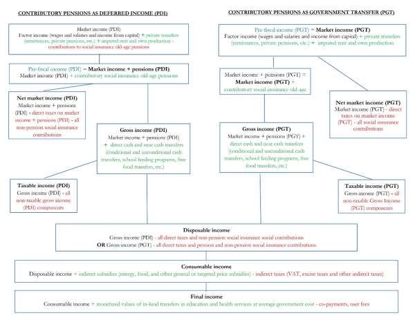
3.2.3. Indirect subsidies

Indirect subsidies (4.9% of GDP) are benefits in the form of reduced prices for specific goods and
services, mainly electricity, gas, and transportation. While many of them are across the board price
subsidies, Tarifa Social provides additional focalized financial help, conditional on some eligibility
requirements.
There are several consumption-price subsidies for electricity and gas. One is a fund financed
through charge on consumer price of gas. These funds are distributed unevenly across regions;
with some subsidized, and others taxed. There are also direct subsidies to gas companies to cover
the cost of price controls. Bottled gas consumption is subsidized for families who do not have
access to the gas network, depending on income and other vulnerability conditions.10
Transportation by train and bus is subsidized. In the case of train, as the state owns the company,
it just charges artificially low prices. In 2017, the state subsidized 50 pesos for each train ticket.
 3.2.4. In-kind transfers

 3.2.4.1. Education

Public schools and universities are financed entirely by the government, and the service is free to
students. Private schools also receive a subsidy from the state, intended to cover professors’
salaries, which are the main cost of the whole system. Primary and secondary education are in the
hands of the provinces, but some financing, such as said subsidies to private schools comes from
national funds. 70% of primary schools across the country receive some kind of state subsidy, and
these institutions account for 93% of primary students. 77% of high schools, accounting for 95%
of high school students, received aid. State financing of education is vast. Argentina ranks second
in expenditure in education as a percentage of GDP in the sample of upper middle-income
countries, with 5.2%, as seen in Figure 4.
 3.2.4.2. Health

In-kind public transfers in health belong to two broad categories: the coverage of the formal
protection system and the public healthcare subsystem.11
The social insurance subsystem includes the National Institute of Social Services for Retirees and
Pensioners (INSSJyPJ). This Institute offers a Comprehensive Medical Assistance Program
(PAMI) to the elderly.
The second component is the coverage of the formal social protection system ―that is, the
coverage for formal workers―, through the social security health insurance system (Obras Sociales),
including both provincial and national plans. Workers (and their employers) also finance this
system through their contributions. As a result, formal workers are entitled to receive a health
insurance plan.

10 There are also supply-side-subsidies to gas, which we are not able to calculate due to the obsolescence of accessible
data, in particular the fact that the most recent input matrix available is from more than a decade ago.
11 For a more detailed description see Gragnolati et al. (2015).

 10

Figure 4. Education expenditure (% of GDP) by country

Source: see Figure 2.

 Figure 5. Health expenditure (% of GDP) by country

Source: see Figure 2.

The public healthcare subsystem consists of subsidized medical attention services provided by
government entities. This is accomplished in two ways: (i) by a supply subsidy structure that

 11

includes hospitals and primary care clinics throughout the country, and (ii) by a program called
Include Health, former Federal Health Care Program (PROFE), that provides coverage to
beneficiaries of non-contributory pensions.
This complex system amounts to nearly 7% of GDP. As we can see in Figure 5, Argentina ranks
first in the size of health spending among comparable countries.
4. Data and methodology

 4.1. Data

The main source of information of the analysis is the household survey Encuesta Permanente de
Hogares (EPH). The EPH is an urban survey that covers 63% of the population and includes
information on household and individual income, cash transfers and personal characteristics
including education and labor market conditions. It does not include information on consumption.
Since our exercise needs to cover the entire population, we assume that the remaining 37% of the
population is similar to those individuals in the survey. We adjust the sampling weights to make
the total population in the survey equal the total population in the country.12
Since Argentina has a medium-high inflation regime, purchasing power can change significantly
throughout a semester. To adjust for inflation, we convert all prices to December 2017’s values.
There is significant item non-response for incomes in the EPH.13 To deal with item non-response
we imputed the missing data applying hot-deck methodology. This method consists of imputing a
missing value from a randomly selected record of individuals with similar characteristics.14
There are also a number of cases of households with zero income. We analyzed their characteristics
to determine whether the income reported is plausible or if it is an error. Most of these households
are inactive individuals, students, under-age, and pensioners who receive the Moratoria or a non-
contributory pension (see Appendix A.1). Hence, we conclude that these reported zero pre-fiscal
incomes are correct.
Since we cannot obtain all the necessary information for the core income concepts from the EPH,
we resort to three complementary surveys. One of them, the 2017/2018 Encuesta Nacional de Gastos
de los Hogares (ENGHo) which collects information on expenditure, income, and characteristics of
households and individuals. The ENGHo is also an urban survey but it expands to as much as
92% of the population.
The second complementary source is the 2015 Encuesta Nacional de Protección y Seguridad Social
(ENAPROSS) which has information on socio-economic characteristics and social protection of

12 This strong assumption is the same approach followed by previous similar efforts (Cruces et al., 2018; Rossignolo,
2018). We leave for future research exploring alternative ways of obtaining information from the population that is
not covered by the EPH.
13 For instance, depending on individual characteristics, the proportion of individuals who did not respond to the

question on main source of income ranges from 12.5% (for salaried workers) to as much as 30.9% (for employers).
14 This was the method used by the Instituto Nacional de Estadísticas y Censos (INDEC) – the Argentine statistical institute

– prior to 2016. Since missing values are imputed, there is no need to reweight the observations, so that we use the
uncorrected base weights (called PONDERA). See also Tornarolli (2018).

 12

households. This survey was collected in the city of Buenos Aires, the Great Buenos Aires, and
villages of at least 5000 inhabitants from five provinces.
The third is the 2009/2010 Encuesta de Movilidad Domiciliaria (ENMODO) for the Área Metropolitana
de Buenos Aires (AMBA), which has information on the characteristics of 22,500 households and
their members and on their mobility and use of public transportation.
Finally, we use national administrative and fiscal information for 2017.
 4.2. Methodology

For some taxes and transfers, the information for how much a household pays or receives is
reported in the EPH. However, direct identification is not always available, so we resort to other
allocation methods as suggested in Lustig (2018). The methods used for each category are
summarized in Table 1 and explained below. In all cases, taxes and transfers were aggregated at
the household level to obtain per capita amounts. For more details, see Appendix A.2.
 4.2.1. Tax allocation

It is assumed that salaried workers and pensioners report their income net of both pension and
non-pension social insurance contributions and personal income tax. For independent workers, it
is assumed that they report income net of only non-pension social insurance contributions.
Therefore, it is not possible to directly identify the burden of direct taxes in the EPH, and we
simulate them based on the contribution and tax rules.
Since the EPH does not have consumption data, direct identification for indirect taxes is not
possible. We use the ENGHo to estimate the burden of the different indirect taxes. Consumption
taxes are assumed to be shifted forward to consumers. Evasion is taken into account implicitly by
using effective rates rather than statutory rates.
 4.2.2. Pensions as deferred income or government transfer (PDI or PGT)

Deciding which way pensions should be treated in Argentina’s case is not straightforward. The
system’s disequilibrium (expenditure minus revenues as a share of revenues) is around 40%
(Cetrángolo & Grushka, 2020). However, 57% of this disequilibrium is explained only by Moratoria,
while the remaining 43% is due to contributory pensions and special regimes. In fact, if we only
consider contributory pensions, the disequilibrium is around 7%.
For practical purposes, in this analysis we take the PDI scenario as closer to Argentina’s situation
in 2017 ―provided we treat the Moratoria as non-contributory and hence as a transfer―, but we
believe the reality lies somewhere in between the two extreme scenarios (the non-contributory
feature of Moratoria, for instance, is an unsolved debate). For this reason, we run both scenarios
(PGT results can be found in the online appendix) and leave the development of a tool that allows
for an incidence analysis in a more realistic hybrid scenario for future research.
 4.2.3. Public spending allocation

In the EPH, one can identify if an individual is receiving a pension, but since contributory and
non-contributory pensions are lumped together, it is not possible to independently identify one

 13

from the other. 15 Thus, we resort to the ENAPROSS to identify the beneficiaries of each type of pension
and then match the pension markers back to the main survey. The amount received is then imputed
according to the law’s rules.
It is not possible to directly identify the beneficiaries of cash transfers in the EPH, and the
availability of information necessary to simulate the impact of each program varies. One question
on the amount received from social programs lumps all of them together. Hence, we take different
approaches and assumptions for each program. Below, we summarize the two most important
direct transfers; for the rest of the programs see. Appendix – Methodology Appendix A.2.
For the AUH we make use of the program’s rules to identify recipients in EPH and simulate the
impact of the program.16 Once identified, we use information on the statutory amount of the
program given to beneficiaries to impute the corresponding value. We only impute the 80%
unconditional part.
For the Moratoria we resort to the ENAPROSS to identify the eligible individuals by decile of the
household per capita income and calculate the ratio of beneficiaries to total amount of pensioners
per decile. Then, for pensioners in each decile in the EPH, we draw a number from a Bernoulli
distribution with probability of success equal to the ratio estimated in the ENAPROSS. The 1s are
considered the beneficiaries of the Moratoria. We also identify as beneficiaries those who declare
to receive a pension if the amount reported is significantly lower than the minimum pension (using
4,000 pesos as the cut-off). We take the reported amount as valid.
It is possible to directly identify students from different levels of education in the EPH.
Expenditure per student is imputed using administrative data on expenditure and on the number
of students. Expenditure per student varies depending on the type of institution (private or public),
province, and education level and it is calculated for each combination of these dimensions.
Since it is not possible to directly identify type of health insurance in the EPH, we use the ENGHo,
where one can identify if an individual has any form of insurance. We define that all the individuals
not reporting having any form of insurance goes to public hospitals. Then, we estimate the
proportion of individuals who have access to each type of health insurance per quintile of per
capita household income. With these proportions, we estimate in the EPH the (rounded) number
of people who have each kind of insurance per quintile of the income per capita distribution.
In the EPH, we assign a random number from a uniform distribution over (0, 1) by which we
order the individuals in each quintile; we then sequentially assign a form insurance until we cover
the estimated proportion of each type. Expenditure per capita is imputed using administrative data
on expenditure and, since there are no official numbers regarding health insurance beneficiaries,
we use the total beneficiaries estimated in the ENGHo (with weights corrected to represent the
total population).
In order to simulate the amount of subsidy (both general and the Tarifa Social) received in each
service, we use the ENGHo in conjunction with the EPH. We first simulate in the EPH potential
beneficiaries of these subsidies by ventile of income per capita and classify them according to
whether or not they are eligible for the Tarifa Social. If they are eligible, we classify them further by

15 Fewer than 1% received both pensions, so we assume that individuals have only one.
16 This has the problem of assuming perfect targeting and no errors of inclusion or exclusion.

 14

the eligibility condition they meet, the number of eligibility conditions they meet, and the region
in which they reside. Then we estimate the quantity of gas and electricity that households consume
in the ENGHo. Since there was considerable noise in the reported quantities consumed, we
estimated the mean quantities consumed by income ventile and region. The size of the subsidies
was estimated as the product of the quantity and imputed subsidy for both the general and the
Tarifa Social component.
5. Results

In this section, we quantify the extent to which the fiscal system impacts overall inequality and
poverty, and identify which components drive the results. To give perspective, we compare
Argentina with other upper middle-income countries from the CEQ Data Center of similar income
per capita: Brazil, Chile, Mexico, Poland, Russia, and Uruguay.17
 5.1. The impact of fiscal policy on inequality and poverty

To see the impact of taxes and transfers on inequality and poverty, we present in Table 2 inequality
measures (Gini coefficient, Theil index, and the 90/10 ratio) and poverty indicators (headcount
ratio, poverty gap index, and squared poverty gap index) with the standard international poverty
lines and the national poverty line.
 Table 2. Inequality and poverty by income concept
 Market income Disposable Consumable Final
 Measure
 + pensions income income income
 Gini 0.477 0.418 0.408 0.308
 Theil index 0.371 0.308 0.293 0.173
 90/10 12.80 7.643 7.204 3.735
 $5.5 per day (2011 PPP) poverty line
 Headcount index 12.4% 6.0% 6.1% Not applicable
 Poverty gap 7.2% 2.2% 2.1% Not applicable
 Sq. poverty gap 5.7% 1.2% 1.1% Not applicable
 National poverty line
 Headcount index 29.5% 22.2% 24.1% Not applicable
 Poverty gap 14.3% 8.1% 8.6% Not applicable
 Sq. poverty gap 9.7% 4.3% 4.4% Not applicable
Source: authors’ own calculations.
Note: these measures are calculated for the PDI scenario. Poverty calculations for final income are not calculated since they would require a
significantly different poverty line (Lustig, 2018).

Argentina’s fiscal system features two characteristics which are desirable for equity in the income
dimension in the short-run. It is overall progressive (reduces inequality), and it lowers poverty.
The redistributive effect of direct and indirect taxes, direct transfers, and subsidies combined is
positive and relatively large comparing with other countries. When pensions are treated as deferred
income, the Gini coefficient declines by 6.9 Gini points.18 Most of the decline occurs through the
effect of direct transfers net of direct taxes. While the combined effect of indirect taxes and
subsidies is still equalizing (something which does not happen in many countries), the size of the
impact is small in comparison. If one also contemplates the impact of transfers in-kind, the fiscal

17 Unless otherwise noted, we present results for the scenario of pensions as deferred income. The results for pensions
as transfers is available in the online appendix.
18 If pensions are considered a government transfer, the redistributive effect rises to 11.1 Gini points.

 15

system is even more equalizing. Compared to the Gini coefficient for consumable income, the
Gini coefficient for final income is 10 points lower. The combined effect of all taxes and all
transfers (including in-kind transfers) leads to a reduction of 16.9 Gini points.
The headcount ratio falls significantly for all poverty lines considered. Generous cash transfers
are the main driver of this result. Even net of direct taxes, the headcount ratio with the $5.5 per
day (2011 PPP) poverty line falls by half of its pre-fiscal level when pensions are treated as deferred
income (and to one third of its pre-fiscal level when pensions are treated as transfers). The marginal
effect of indirect taxes and subsidies on poverty (the difference between disposable and
consumable income headcount) is nil when using the international poverty lines. When poverty is
measured with the national poverty line, the effect is poverty increasing.
Net payers to the fiscal system are those who live in households that receive less in transfers and
subsidies than they pay in taxes – i.e., those whose consumable income is lower than pre-fiscal
income. Net payers in Argentina start at the 6th decile and the more than $10 per day (2011 PPP)
income category, which means that the extreme poor, moderate poor, and vulnerable to poverty
groups are net receivers.19 Argentina stands out by this high number of net receivers compared
with Brazil 2009 (3rd decile), Mexico 2014 (4th decile), and Uruguay 2009 (3rd decile). In Chile and
Russia, net payers also start at the middle class.
The estimated reduction in inequality and poverty is quite large, especially compared with the other
upper middle-income countries, as Table 3 shows. While these results put Argentina seemingly in
a bright spot, we will see that the main factor behind these results is the amount of public spending
and not its overall progressivity. Tax revenues are quite high, and yet not enough to keep up with
problematic spending levels. Even though not the direct focus of our analysis, we cannot finish a
section on the impact of fiscal policy on poverty without taking these effects into consideration.
Fiscal imbalances have been a key cause in subsequent recessions in recent Argentine
macroeconomic history.20 In the two-year period 2018-2019, GDP per person fell by 3%. The
incidence of poverty rose 8.2 percentage points from 27.3 to 35.5% between the first semester of
2018 and the second semester of 2019 (INDEC, 2020). Using the same metric of national poverty
line and disposable income, the headcount ratio fell by 6.4 percentage points as a result of direct
transfers (net of taxes). That is, the recession caused poverty to rise in two years by more than the
fiscal system reduced it in 2017. This suggests that redistributive policies can be self-defeating if
not anchored in a fiscally prudent framework.
 5.2. Determinants: size, progressivity and reranking

The extent of fiscal redistribution and poverty reduction depends on the size and progressivity of
the fiscal system. To see which factor is more important in the Argentine case we use Lambert
(2001)’s equation for the overall progressivity of the fiscal system, which equals a weighted sum of
the progressivity of taxes and transfers:

 ( + 
 )
 =
 (1 – + )

19 Income categories income are standard definitions based on dollars per day (2011 PPP).
20 See, for instance, Llach & Gerchunoff (2018), Mussa (2002), and Sturzenegger (2019).

 16

Table 3. Inequality and poverty by country
 Market income Disposable Consumable Final
 Country
 + pensions income income income
 Gini coefficient
 Argentina 17’ 0.477 0.418 0.408 0.308
 Brazil 08’ 0.573 0.545 0.542 0.430
 Chile 13’ 0.494 0.467 0.464 0.419
 Mexico 14’ 0.528 0.494 0.492 0.393
 Poland 14’ 0.412 0.345 0.355 0.291
 Russia 10’ 0.379 0.348 0.351 0.299
 Uruguay 08’ 0.505 0.467 0.468 0.377
 $5.5 per day (2011 PPP) poverty line
 Argentina 17’ 12.4% 6.0% 6.1% Not applicable
 Brazil 08’ 32.0% 30.3% 35.7% Not applicable
 Chile 13’ 8.3% 5.3% 6.7% Not applicable
 Mexico 14’ 36.3% 36.1% 37.4% Not applicable
 Russia 10’ 6.9% 4.9% 5.9% Not applicable
 Uruguay 08’ 15.9% 11.5% 15.0% Not applicable
 Source: see Figure 2.
 Note: data for Poland not available.

where is the Reynolds-Smolensky (RS) index of progressivity of the fiscal system (“Vertical
Equity”). In the absence of reranking, RS is identical to the difference between the post-fiscal and
pre-fiscal Gini coefficients. g and b are the ratio of taxes and transfers to pre-fiscal income, and
 and are the Kakwani indexes for total taxes and total transfers. This equation can be used
 21

to compare the relative importance of size versus progressivity (in the absence of reranking, which
we shall assume away for now in analyzing the drivers of fiscal redistribution).
Measured by the ratio of social spending to GDP (even leaving out contributory pensions),
Argentina’s fiscal system is the largest among similar countries (Figure 6).
Regarding progressivity as measured by the Kakwani index, Table 4 shows that direct taxes in
Argentina are the least progressive except for Russia. Indirect taxes are the most regressive in
Argentina. All taxes combined are regressive only for Argentina.22 Direct transfers are relatively
progressive but less so than in Uruguay, Mexico, and Chile, while subsidies are the least
progressive. In the case of education spending, Argentina is among the most progressive. For
health, the country is among the less progressive group.
Thus, the large impact on inequality and poverty observed in Argentina is primarily driven by the
large amount of resources devoted to social spending and subsidies. The poor performance in
terms of progressivity on some of the spending components must mean that a nontrivial portion
of resources is spent on the non-poor. As we shall see, this is particularly true for subsidies.
Beyond low progressivity, another factor that can weaken the redistributive power of taxes and
transfers is the presence of reranking. Reranking, the swapping of individuals in the distribution,
is considered a measure of horizontal inequity and of “waste” in the redistributive machinery. The
reranking effect for all taxes and transfers equals 0.022. To put this in perspective, we take the

21 The Kakwani index for tax (transfer) is defined as the (negative of the) difference between the concentration
coefficient for the tax (transfer) in question and the Gini coefficient. A positive (negative) Kakwani index means that
the tax or transfer is progressive (regressive).
22 We carried out a sensitivity analysis to uncover the reasons behind this seemingly odd feature and found that a main

driver of this result is the existence of a quite special program: Moratoria. For more details, see Appendix A.1.

 17

ratio of this effect to the redistributive and the vertical equity effects. These ratios equal 13% and
12%. Comparing with other countries in Table 5 we observe that the extent of reranking is much
lower than Russia’s, much higher than Uruguay, and similar to Brazil, Chile, and Mexico.
Argentina’s fiscal system does not seem to feature more reranking than comparable countries.23
 Figure 6. Social spending and subsidies (% of GDP) by country

Source: see Figure 2.
Notes: social spending includes expenditure on direct transfers, education, health and other social spending. It does not include contributory
pensions. Indirect subsidies not available for Poland, Brazil, Russia, and Uruguay.

 Table 4. Kakwani index by country
 Kawkani Index
 Gini
 Country Direct Direct Indirect All SS +
 coefficient Subsidies Education Health
 taxes transfers taxes taxes subsidies
 Argentina 17' 0.477 0.132 0.738 -0.088 0.352 -0.021 0.633 0.489 0.578
 Brazil 08' 0.573 0.169 0.464 -0.025 0.712 0.046 0.711 0.690 0.647
 Chile 13' 0.494 0.143 0.824 -0.027 0.497 0.025 0.664 0.592 0.674
 Mexico 14' 0.528 0.167 0.852 -0.005 0.060 0.104 0.608 0.466 0.539
 Russia 10' 0.379 0.116 0.594 -0.066 0.173 0.020 0.510 0.371 0.472
 Uruguay 09' 0.505 0.151 0.979 -0.050 n.a.. 0.042 0.668 0.608 0.684
 Average 0.493 0.146 0.742 -0.043 0.359 0.036 0.633 0.536 0.599
Source: see Figure 2.
Notes: n.a.= not available. Gini coefficient is calculated for market income + pensions. Data for Poland not available.

 There are countries in which the reranking effect is so large that it takes away the entire redistributive effect. In the
23

CEQ Data Center sample, this occurs in Bolivia and Indonesia.

 18

Table 5. Redistributive, Vertical Equity and Reranking Effects by country

 Redistributive Vertical Equity Reranking Reranking Reranking
 Country
 Effect (RE) Effect (VE) Effect over RE over VE
 Argentina 17' 0.169 0.192 0.022 13% 12%
 Brazil 08' 0.143 0.158 0.015 10% 9%
 Chile 13' 0.075 0.084 0.009 12% 10%
 Mexico 14' 0.135 0.151 0.016 12% 11%
 Russia 10' 0.080 0.105 0.025 32% 24%
 Uruguay 09' 0.128 0.135 0.007 5% 5%
 Average 0.122 0.137 0.010 14% 12%
 Source: see Figure 2.
 Note: data for Poland not available.

 5.3. Components of the fiscal system: marginal contributions, pro-poorness, and
 leakages to the non-poor

The previous section analyzed the determinants of the broad redistributive effect of the Argentine
fiscal system. In this section, using marginal contributions24, we focus on identifying which specific
taxes, transfers, and subsidies contribute the most to the reduction in inequality and poverty and
which ones are most unequalizing. We also assess which specific transfers are more targeted to the
poor and which ones allocate an inordinate amount of resources to the non-poor. For this purpose,
we will look at the concentration coefficients and concentration shares by income category.
Table 6 shows that the spending interventions which contribute more to reducing inequality are
the Moratoria, the PNC, and the AUH. These are also the programs that contribute the most to
reduce poverty. These results are not surprising because the first two programs are non-
contributory pensions whose beneficiaries are likely to have zero or very low pre-fiscal incomes.25
Subsidies are equalizing but to a much lower extent. They are also poverty reducing. One aspect
to note is that the marginal contribution of subsidies to poverty reduction increases as we measure
it with higher poverty lines. This is telling us that subsidies benefit the moderate poor relatively
more than the extreme poor. Regarding in-kind transfers, the most equalizing is public health care
and primary and secondary education, in that order. The least equalizing is spending on tertiary
education.26
On the tax side, excise taxes, fuel taxes, and value added taxes are outright unequalizing. The most
equalizing tax is personal income tax. All taxes by definition are poverty increasing, but the value
added tax has the highest marginal contribution and by a nontrivial difference from the next in
line. The value added tax is significantly poverty increasing for poverty measured by low or higher
poverty lines, as shown in the Table 6.

24 The marginal contribution of a tax (transfer) is calculated by taking the difference between inequality (or poverty)
indicator without the tax (transfer) and with it.
25 Incidence of these programs is broken down by deciles in Figures A3 through A5 in the Appendix A.3. Although

incidence as a percentage of pre-fiscal income declines with income for all three programs, incidence in dollars per
capita only falls monotonically with income for the AUH and remains constant after the first decile for the PNC and
Moratoria.
26 See figures A6 through A11 in the Appendix A.3.

 19

Regarding payroll taxes, there are concerns about its progressivity. Despite being less so than
personal income tax, they are progressive and equalizing, unlike indirect taxes. Figure A.12 in the
Appendix A.3 shows that the higher deciles are the ones who pay most of these taxes.
We consider pro-poor those spending categories that have negative concentration coefficients –
per person spending declining with income. The more a program is targeted to the poor, the more
negative the concentration coefficient will be. In Table 6 we see that the pro-poor spending
categories are (in decreasing order) the AUH, Moratoria, bottled gas subsidy, Capacitación y Empleo,
JMyMT (youth program), scholarships, PNC, unemployment insurance, community kitchens, and
bus subsidies.
 Table 6. Marginal Contributions by program

 Redistribution Poverty reduction
 Size (% of Marginal
 Concentration Kakwani MC MC MC
Budget item market income Contribution
 coefficient index $3.2 $5.5 national
 + pensions) (MC)
Disposable income 105.2%
Direct transfers 11.0% -0.261 0.738 0.051 0.056 0.065 0.082
Moratoria 5.4% -0.338 0.815 0.021 0.023 0.026 0.035
PNC 2.5% -0.222 0.699 0.013 0.017 0.019 0.021
AAFF 1.5% 0.076 0.401 0.005 0.000 0.001 0.010
AUH 1.1% -0.533 1.010 0.011 0.019 0.021 0.012
Progresar 0.2% 0.053 0.424 0.001 0.001 0.001 0.001
Community kitchens 0.2% -0.002 0.479 0.001 0.001 0.000 0.002
UI 0.1% -0.046 0.523 0.000 0.001 0.001 0.001
Scholarships 0.0% -0.221 0.698 0.000 0.000 0.001 0.001
JMyMT 0.0% -0.248 0.725 0.000 0.000 0.000 0.000
Capacitación y Empleo 0.0% -0.287 0.764 0.000 0.000 0.000 0.000
Direct taxes 5.8% 0.609 0.132 0.008 -0.000 -0.002 -0.010
Personal income tax 2.1% 0.762 0.285 0.006 0.000 0.000 -0.001
Health contributions 2.6% 0.524 0.047 0.001 -0.000 -0.001 -0.007
Payroll taxes 1.1% 0.524 0.047 0.000 -0.000 -0.000 -0.003
Consumable income 96.7%
Subsidies 4.6% 0.125 0.352 0.015 0.023 0.018 0.027
Electricity subsidy 2.5% 0.177 0.300 0.007 0.007 0.007 0.015
Gas subsidy 0.9% 0.214 0.263 0.002 0.002 0.002 0.005
Bus subsidy 0.8% -0.016 0.493 0.004 0.004 0.005 0.007
Bottled gas subsidy 0.2% -0.317 0.794 0.002 0.003 0.003 0.004
Train subsidy 0.2% 0.139 0.338 0.007 0.001 0.000 0.001
Indirect taxes 13.1% 0.389 -0.088 -0.014 -0.015 -0.032 -0.063
Value added tax 8.7% 0.382 -0.095 -0.009 -0.008 -0.0194 -0.041
Fuel taxes 0.7% 0.279 -0.198 -0.001 -0.001 -0.002 -0.004
Excise taxes 1.1% 0.307 -0.170 -0.002 -0.001 -0.002 -0.007
IIBB tax 2.5% 0.477 -0.000 -0.000 -0.001 -0.0023 -0.009
Final income 122.4%
In-kind transfers 25.3% -0.072 0.549 0.106 Not app. Not app. Not app.
Initial education 1.0% -0.230 0.708 0.007 Not app. Not app. Not app.
Primary education 3.5% -0.264 0.741 0.023 Not app. Not app. Not app.
Secondary education 4.1% -0.195 0.672 0.024 Not app. Not app. Not app.
Tertiary education 1.9% 0.160 0.317 0.005 Not app. Not app. Not app.
PAMI 2.0% 0.033 0.444 0.008 Not app. Not app. Not app.
Social security health insurance 6.7% 0.106 0.372 0.023 Not app. Not app. Not app.
Public health care 6.0% -0.155 0.632 0.035 Not app. Not app. Not app.
Source: authors’ own calculations.
Note: see Tables 1 and 2.

While the concentration coefficient gives us a summary measure of pro-poorness, it does not allow
us to see the extent to which resources are allocated to the non-poor. In Table 7 we show the
concentration shares by income category – the ultra, extreme, and moderate poor, the vulnerable

 20