Genotype-specific P-spline response surfaces assist interpretation of regional wheat adaptation to climate change
←
→
Page content transcription
If your browser does not render page correctly, please read the page content below
in silico Plants Vol. 3, No. 2, pp. 1–23
https://doi.org/10.1093/insilicoplants/diab018
Advance Access publication 06 July 2021
Special Issue: Linking Crop/Plant Models and Genetics
Original Research

                                                                                                                                                                                           Downloaded from https://academic.oup.com/insilicoplants/article/3/2/diab018/6316219 by Wageningen University en Research -Library user on 08 October 2021
     Genotype-specific P-spline response surfaces assist
       interpretation of regional wheat adaptation to
                       climate change
   Daniela Bustos-Korts1,* , , Martin P. Boer1, Karine Chenu2, , Bangyou Zheng3, ,
                   Scott Chapman2,4 and Fred A. van Eeuwijk1
                                         1
                                          Biometris, Wageningen University and Research, 6708 PB Wageningen, The Netherlands
                     2
                         Queensland Alliance for Agriculture and Food Innovation, The University of Queensland, Queensland, QLD 4072, Australia
                                                3
                                                 CSIRO Agriculture and Food, Brisbane, Queensland, QLD 4067, Australia
                               4
                                 School of Agriculture and Food Sciences, The University of Queensland, Queensland, QLD 4343, Australia
                                                    *Corresponding author’s email address: daniela.bustoskorts@wur.nl

                                                        Guest Editor: Carlos Messina; Editor-in-Chief: Stephen P Long

Citation: Bustos-Korts D, Boer MP, Chenu K, Zheng B, Chapman S, van FA. 2021. Genotype-specific P-spline response surfaces assist interpretation of regional
                           wheat adaptation to climate change. In Silico Plants 2021: diab018; doi: 10.1093/insilicoplants/diab018

                                                                                     A B ST R A CT
                  Yield is a function of environmental quality and the sensitivity with which genotypes react to that. Environmental
              quality is characterized by meteorological data, soil and agronomic management, whereas genotypic sensitivity
              is embodied by combinations of physiological traits that determine the crop capture and partitioning of envi-
              ronmental resources over time. This paper illustrates how environmental quality and genotype responses can be
              studied by a combination of crop simulation and statistical modelling. We characterized the genotype by environ-
              ment interaction for grain yield of a wheat population segregating for flowering time by simulating it using the
              the Agricultural Production Systems sIMulator (APSIM) cropping systems model. For sites in the NE Australian
              wheat-belt, we used meteorological information as integrated by APSIM to classify years according to water, heat
              and frost stress. Results highlight that the frequency of years with more severe water and temperature stress has
              largely increased in recent years. Consequently, it is likely that future varieties will need to cope with more stress-
              ful conditions than in the past, making it important to select for flowering habits contributing to temperature and
              water-stress adaptation. Conditional on year types, we fitted yield response surfaces as functions of genotype, lati-
              tude and longitude to virtual multi-environment trials. Response surfaces were fitted by two-dimensional P-splines
              in a mixed-model framework to predict yield at high spatial resolution. Predicted yields demonstrated how relative
              genotype performance changed with location and year type and how genotype by environment interactions can
              be dissected. Predicted response surfaces for yield can be used for performance recommendations, quantification
              of yield stability and environmental characterization.

              K E Y W O R D S : Adaptation landscape; APSIM; breeding strategy; climate change; G×E; P-splines; wheat.

                           1. INTRODUCTION                                                        plant breeders evaluate their candidate varieties (genotypes) in a set of
Genotypes vary in their sensitivity to the environmental conditions,                              multi-environment trials (METs). Multi-environment trials aim to repre-
which is the basis for their improvement by plant breeding. These differ-                         sent the growing conditions that varieties are likely to encounter when
ences in sensitivity lead to genotype by environment interaction (G×E),                           grown by farmers. This set of conditions is usually described as the target
potentially changing the genotypic ranking across levels of environmental                         population of environments (TPE; Comstock and Moll 1963; Chapman
quality. To understand G×E, and to make genotype recommendations,                                 et al. 2000b; Chenu 2015; Hammer et al. 2019).

© The Author(s) 2021. Published by Oxford University Press on behalf of the Annals of Botany Company.
This is an Open Access article distributed under the terms of the Creative Commons Attribution License (http://creativecommons.org/licenses/by/4.0/), which permits unrestricted
                                                                                                                                                                                   •   1
reuse, distribution, and reproduction in any medium, provided the original work is properly cited.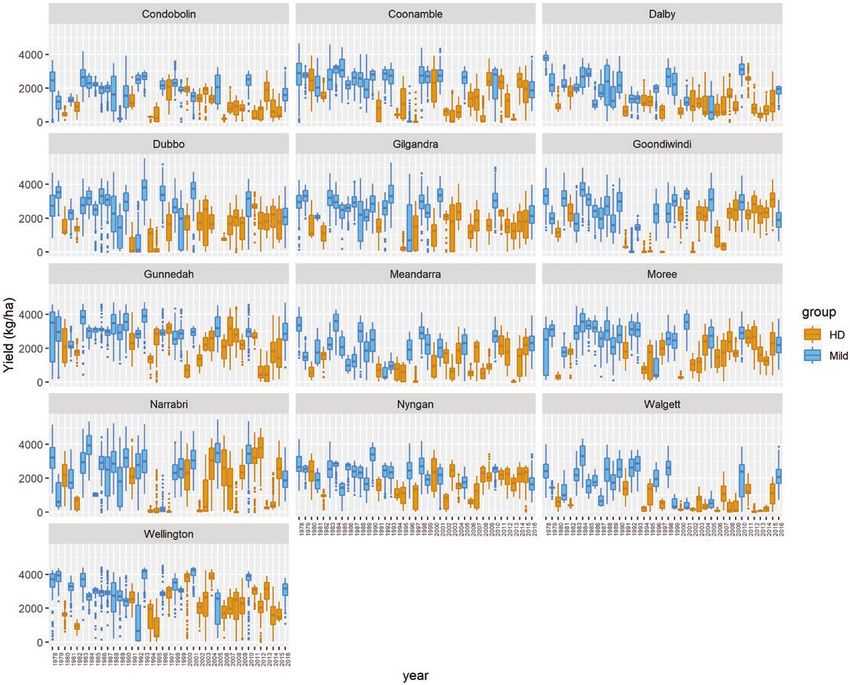
2   •   Genotype-specific P-spline response surfaces

    Locations used for the METs are a sample of possible locations                  The choice of which environmental covariables to include in the
that belong to the TPE. Hence, breeders and farmers are not only               prediction model largely depends on the environmental drivers for
interested in characterizing adaptation to those specific locations, but       G×E. Within the TPE sample represented by METs, there may be
across the whole latitude and longitude range encompassed by the               recurring or repeating characteristics (i.e. that remain constant across

                                                                                                                                                                Downloaded from https://academic.oup.com/insilicoplants/article/3/2/diab018/6316219 by Wageningen University en Research -Library user on 08 October 2021
TPE. With this aim, genotype adaptation needs to be predicted across           years for a given location) that induce differential genotypic responses,
the whole range of geographies in which genotypes will potentially be          which are an expression of G×E. Typical repeating characteristics are
grown (Cooper et al. 2014). Across the TPE, a given genotype shows             associated with latitude, longitude and to soil type. Latitude usually has
adaptation to the region in which it realizes highest yields, and for a        a large effect on differential genotype adaptation via its effect on phe-
given region, the highest yielding genotype shows the best adapta-             nology (Zheng et al. 2012, 2013), whereas soil characteristics largely
tion to that region (van Eeuwijk et al. 2016). Predictions of genotype         impact nutrient and water availability for the crop. Hence, soil differ-
performance across the TPE can be made for subsets of locations                ences between locations are usually increased in environments with
that are internally homogeneous, called mega-environments (Atlin               low rainfall (Wang et al. 2017). Note, however, that in real-world METs,
et al. 2000; Piepho and Möhring 2005; Chauhan et al. 2017). Mega-              the effects of ‘location’ may be affected by the fact that a ‘location’ refer-
environments can be geographically defined by subsets of locations             ence is usually associated with a nearby geographical reference (such as
that share weather or soil characteristics, and these locations may not        a town name), and the actual trials are not done in the exact same field
be contiguous or adjacent, especially when considered in a national or         each year even if breeders try to choose a typical soil type and man-
global context. In dry environments as those in the Australian wheat-          agement. In low-rainfall environments like Australia where fallows and
belt, soil characteristics can largely determine the level of water stress,    crop rotations are common, running a trial in exactly the same field and
as they influence water retention capacity (Chenu et al. 2013). Besides        same place in successive years would be considered poor experimental
describing environments as instances of mega-environments, environ-            practice due to potential carry-over effects of plot effects, impacts on
ments can be described as functions of explicit environmental gradi-           soil water reserves and pressure of weeds and diseases.
ents, represented by latitude and longitude (Lowry et al. 2019). As an              Other characteristics of environmental quality are less predict-
extension of this latter approach, latitude and longitude can be com-          able because they change from year to year with the weather fluc-
plemented and replaced by explicit environmental covariables related           tuations, but they are predictable from their frequencies estimated
to weather or agronomic management (Malosetti et al. 2004; Millet              from long-term data. For example, the long-term frequency of water
et al. 2016).                                                                  supply-demand ratio (Chapman et al. 2000b; Chenu et al. 2013) and
    There is a range of possible models to predict genotype adapta-            the frequency of El Niño–Southern Oscillation (ENSO) events in the
tion across a gradient defined either by geographical coordinates or by        eastern Australian wheat-belt (Zheng et al. 2018) could potentially be
explicit environment quality (Piepho and Möhring 2005; Smith et al.            used to estimate the probability of a certain stress level to occur at a
2005; van Eeuwijk et al. 2005, 2019; Piepho et al. 2014; Bustos-Korts          particular location. If the probability of a certain year type (weather
et al. 2016). For example, the factorial regression models are a linear        scenario) can be estimated from long-term data, it becomes attractive
function of the genotypic sensitivities to environmental covariables,          to predict response surfaces across latitude and longitude for each of
and are popular due to their simplicity and because their parameters           the likely weather scenarios across years. In that way, latitude and lon-
offer a clear biological interpretation in terms of genotype average           gitude effects become repeatable G×E, conditional on a year type or
performance and sensitivity to the environment (Cullis et al. 1996;            weather scenario.
Brancourt-Hulmel et al. 2000; Malosetti et al. 2004, 2013; Smith et al.             In Australia, national variety trials of wheat are conducted by the
2005; Millet et al. 2016; Parent et al. 2017; Bustos-Korts et al. 2018).       GRDC (Grains Research and Development Corporation) in coop-
    While factorial regression models are a convenient approach to pre-        eration with commercial breeding companies. Those companies also
dict adaptation across an environmental gradient, they may be restric-         conduct their own research trials. However, in neither of these vari-
tive in cases where gradient effects are non-linear, as it is often the case   ety trials are the same varieties grown over large numbers of seasons.
in plant breeding. To fit non-linear responses, factorial regression mod-      The limited replication of varieties over years represents a bottleneck
els can be extended to include quadratic or higher order polynomial            in studying long-term adaptative responses. This bottleneck can be
terms, but this will require large numbers of degrees of freedom with          addressed by utilizing crop simulation models to construct synthetic/
consequent problems in fitting. Spline models offer a flexible alterna-        virtual breeding trial data sets that span a longer series of years. This
tive to model non-linear responses (Eilers and Marx 1996; Eilers et al.        approach has been widely adopted for multiple crops; e.g. sorghum
2015), and can be even extended to model variation across multiple             (Chapman et al. 2002; Hammer et al. 2014, 2019), maize (Chenu et al.
dimensions (Lee et al. 2013; Wood et al. 2013; Rodríguez-Álvarez et al.        2009; Harrison et al. 2014; Messina et al. 2011), wheat (Chenu et al.
2015; Wood 2017). Two-dimensional P-spline models are being used               2017) and soybean (Messina et al. 2006), including studies that look
to separate genetic differences from spatial heterogeneity within trials       at flowering time effects in wheat for current (Zheng et al. 2015b) and
(Velazco et al. 2017; Rodríguez-Álvarez et al. 2018; Boer et al. 2020).        future climates (Zheng et al. 2016).
In this paper, we aim to illustrate the use of two-dimensional P-spline             In this paper, we present the use of P-splines embedded in mixed
approaches at larger scales than trials, i.e. to model spatially dependent     models to interpret G×E and predict the adaptive responses of indi-
G×E variation at the level of the TPE, predicting the yield response           vidual wheat genotypes from simulated data for a region of about 677
surfaces of individual genotypes as a function of only latitude and            by 445 km in size. The Agricultural Production Systems sIMulator
longitude.                                                                     (APSIM) yield was simulated for 156 genotypes varying in flowering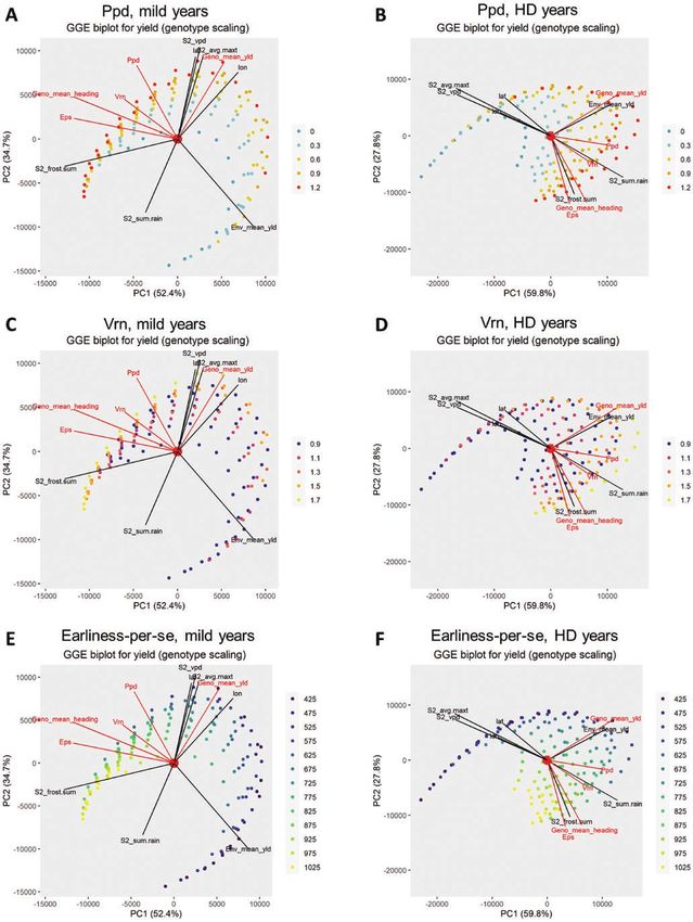
Bustos-Korts et al. • 3
time and sown in 13 Australian locations across 39 years of weather 2. METHODS
records. We focus on the adaptive responses across latitude and longi- This section describes the main steps of our approach; data genera-
tude, and we examine how these response surfaces change depending tion using simulations in APSIM Wheat, G×E analysis of outputs gen-
on the level of drought and heat stress present across years. We also erated by APSIM and construction of environmental indices using
Downloaded from https://academic.oup.com/insilicoplants/article/3/2/diab018/6316219 by Wageningen University en Research -Library user on 08 October 2021
describe the adaptation landscape in terms of the traits contributing APSIM outputs to facilitate classification of years in year types.
to adaptation across environmental conditions (i.e. sensitivity to pho- Conditional on year type, yield response surface models for individ-
toperiod, vernalization requirements and thermal time requirements ual genotypes were fitted as functions of longitude and latitude using
from floral initiation and flowering). P-spline methods within a mixed-model context. The fitted response
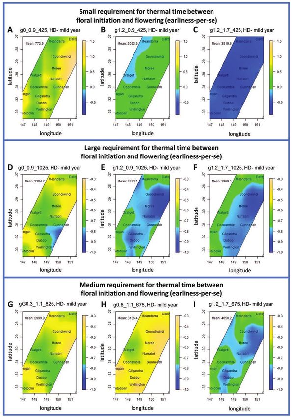
Figure 1. General overview of the modelling approaches used to generate the APSIM yield data, fitting of P-splines and generating
predictions along the whole latitude–longitude surface, and use of P-spline predictions to classify locations.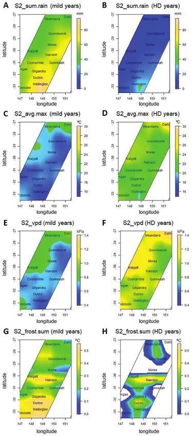
4   •   Genotype-specific P-spline response surfaces

surfaces provided predictions of yield responses at any desired reso-    indicates the minimum thermal time requirement from floral initia-
lution level for all genotypes. The yield predictions were used to       tion to flowering. For example, ‘g1.2_0.9_425’ indicates a genotype
subdivide the area defined by longitude and latitude coordinates in      with a sensitivity to photoperiod of 1.2, vernalization requirements
adaptation zones. Our workflow is schematically represented in Fig. 1.   of 0.9 and minimum thermal time requirement from floral initia-

                                                                                                                                                  Downloaded from https://academic.oup.com/insilicoplants/article/3/2/diab018/6316219 by Wageningen University en Research -Library user on 08 October 2021
                                                                         tion to flowering of 425 °Cd. For most of the environments, the
                      2.1 Simulated data                                 range for flowering time was around 50 days [see Supporting
Data corresponded to grain yield for 156 wheat genotypes simu-           Information—Fig. S5]. Note that this genotypic variation can
lated by Zheng et al. (2018) using the APSIM cropping system             be considered to be rather extreme compared to real-world con-
model (Holzworth et al. 2014) together with a phenology model            ditions. Australian breeders tend to select wheats for early-season
(Zheng et al. 2013), frost impact module (Zheng et al. 2015a) and        (slower maturing) or main-season (faster maturing) sowing times.
heat impact module (Lobell et al. 2015). In this data set, variation     Commercial wheats are often classified as ‘quick’, ‘medium’ or ‘slow’
in APSIM genotype-specific parameters was induced by allelic vari-       and are usually compared to reference cultivars that are established
ation for the VRN-A1, VRN-B1, VRN-D1 and PPD-D1 genes, and               on the market. Consequently, the range in flowering time within a
the full range of values of additional thermal time requirements         typical breeders trial may be 3–4 weeks in early generation breed-
from floral initiation to flowering (from 425 to 1025 °Cd; Zheng         ing, or 1–3 weeks in the type of MET we are considering here, i.e.
et al. 2013). The set of genotypes included commercial varieties         much less than 50 days.
and virtual genotypes that could potentially be bred based on the            In this study, we focused on 13 out of the 15 locations used in
flowering alleles present in the Australian germplasm pool (Zheng        Zheng et al. (2018), removing ‘Emerald’ and ‘Roma’ (Fig. 2; Table
et al. 2013). Allelic combinations at vernalization and photoperiod      1). We dropped Emerald because it was geographically too distant,
genes produced variation for the APSIM parameters; Ppd, Vrn and          which does not allow for a reliable surface estimation with P-splines.
Eps. Genotypes with the same phenology (but different allelic            Roma had extreme stress conditions, leading to zero yield for many
combinations) were disregarded, so that a total of 156 genotypes         genotypes. For the 13 locations we considered, yield was simulated
unique for their phenology were considered. Overall, the selected        for each season from 1978 to 2016. Zheng et al. (2018) simulated
genotypes had APSIM parameters ranging from 0 to 1.2 for the             several sowing dates. In this study, we restricted ourselves to one
photoperiod sensitivity (Ppd parameter, with values of 0, 0.3, 0.6,      sowing date per location (the same date was used across years). The
0.9 and 1.2, with 0.6 for the reference genotype Janz), 0.9 to 1.7 for   selected sowing date per location was identified as the one leading
the vernalization sensitivity (Vrn parameter, with values of 0.9, 1.1,   to the largest yield for the average of the genotypes (‘optimal’ sow-
1.3, 1.5 and 1.7, with 0.9 for Janz) and 425 to 1025 °Cd for earli-      ing date; Table 1). For a location, the starting soil conditions were
ness-per-se (Eps parameter, with values of 425, 475, 525, 575, 625,      the same in every year of simulation and represented the average
675, 725, 775, 825, 925, 975 and 1025 °Cd, with 675 °Cd for Janz).       starting condition for that location after the analysis of historical
Genotypes were labelled by their flowering time parameters; the          data in Zheng et al. (2018). Four environments with a large crop
first number indicates the value for sensitivity to photoperiod, the     failure were removed, leaving in total 503 environments for the G×E
second indicates vernalization requirement and the third number          analysis.

Figure 2. Trial locations used to simulate APSIM yield between 1978 and 2016.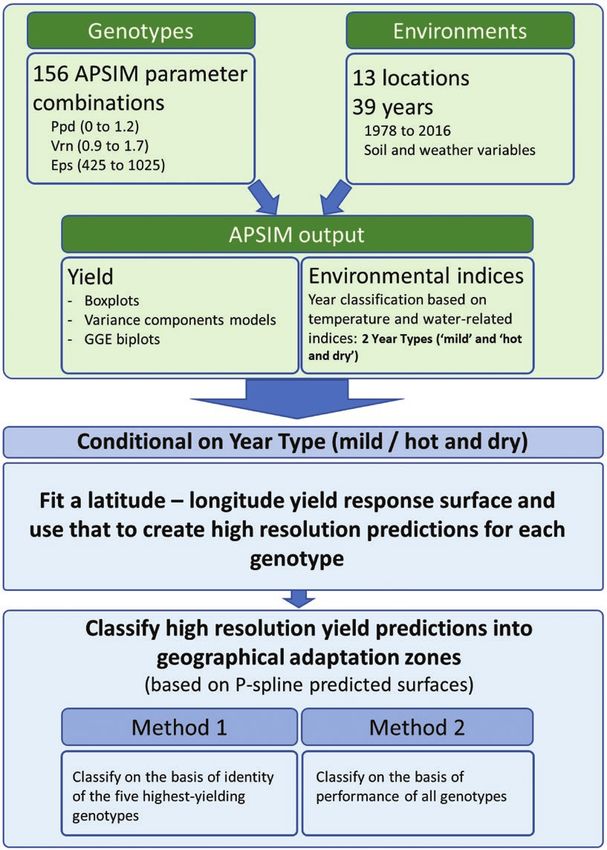
Bustos-Korts et al.    •    5

Table 1. Location name, latitude, longitude and sowing date for the 13 locations considered in this study with their
corresponding mean simulated yield and date to flowering together with their corresponding standard deviations (SDs) across
genotypes and years. Data simulated for 156 genotypes differing in phenology, over 1978–2016. QLD, Queensland; NSW, New
South Wales.

                                                                                                                                                          Downloaded from https://academic.oup.com/insilicoplants/article/3/2/diab018/6316219 by Wageningen University en Research -Library user on 08 October 2021
State     Region                       Name               Latitude       Longitude      Sowing date            Days to             Yield (kg ha−1)
                                                                                                              flowering
                                                                                                           Mean        SD         Mean           SD
QLD       Eastern Darling Downs        Dalby               -27.18         151.26        29 May             114.1      13.5       1593.3          942.4
QLD       Western Darling Downs        Meandarra           -27.32         149.88        7 May              115.7      16.1       1578.6         1034.0
QLD       Western Darling Downs        Goondiwindi         -28.55         150.31        11 April           107.2      20.7       2000.8         1180.3
NSW       Northern NSW                 Moree               -29.48         149.84        5 May              121.7      16.7       2141.6         1048.8
NSW       Northern NSW                 Walgett             -30.04         148.12        5 May              121.5      16.4       1205.7         1054.4
NSW       Northern NSW                 Narrabri            -30.32         149.78        21 April           121.0      19.6       2005.5         1440.6
NSW       Northern NSW                 Coonamble           -30.98         148.38        21 April           124.3      19.7       1838.7         1125.0
NSW       Eastern NSW                  Gunnedah            -30.98         150.25        5 May              127.7      16.7       2504.1         1024.0
NSW       Western NSW                  Nyngan              -31.55         147.20        17 April           123.4      20.6       1959.7          819.6
NSW       Western NSW                  Gilgandra           -31.71         148.66        25 April           143.4      18.7       2115.9         1047.1
NSW       Western NSW                  Dubbo               -32.24         148.61        29 April           140.9      17.8       2073.4         1167.1
NSW       Eastern NSW                  Wellington          -32.80         148.80        23 April           156.1      18.6       2593.8         1066.1
NSW       Western NSW                  Condobolin          -33.07         147.23        11 May             139.4      16.0       1447.3          883.0

2.2 Using environmental covariables to classify years                     years as objects in rows and index–location combinations as variables
                 into year types                                          in columns. Variables were centred and scaled, and were used to calcu-
Water and temperature stress are common environmental drivers for         late Euclidean distances between years. These distances were used in a
grain yield in Australian wheat production systems (Chenu et al. 2011,    hierarchical clustering procedure to classify years according to the four
2013; Ababaei and Chenu 2020). To help classifying years according        environmental indices relating to water, frost and heat stress (Ward
to their water and temperature stress, we used APSIM to compute four      method; Zelterman 2015) using the ‘hclust’ function in R (R Core
environmental indices for each genotype (Table 2; see Supporting          Team 2019). With this clustering procedure, years were classified into
Information—Figs S2–S4). These indices were related to water, frost       two classes; ‘mild’ years (with reduced water and temperature stress)
and heat stress. Indices were calculated between 300 °Cd before flow-     and ‘hot and dry’ (with water, frost and heat stress).
ering and 100 °Cd after flowering, coinciding with the critical period
for grain number determination (Table 2).
                                                                                         2.3 Mixed-model G×E analysis
    After computing the indices per genotype, we averaged the values
                                                                          2.3.1 Variance components model To quantify the relative contribu-
across all genotypes for each year–location combination. The aver-
                                                                          tion of locations and years to the total G×E, we fitted the following
age environmental indices across genotypes were used to character-
                                                                          mixed model to the APSIM yield:
ize environmental quality. Then, data were arranged in a matrix with
                                                                          y = µ + Lj + Yk + LYjk + Gi + GLij + GY ik + GLY ijk
                                                                          (1)
                                                                           ijk

Table 2. Description of the environmental indices                         In equation (1), y is the phenotype (yield) of the ith genotype in
calculated with APSIM output and that were used to                                           ijk
                                                                          the jth location and the kth year (i = 1,...156; j = 1,...13; k = 1,...39).
classify environments according to their levels of water and
temperature stress. The four indices were calculated in a period          µ is the general intercept, Lj and Yk are the fixed effects of location
from flowering + 100 °Cd to flowering + 600 °Cd.                          and year and LYjk is the fixed interaction between location and year.

Name environmental index         Description                              Gi is the random main effect of the ith genotype, whereas GLij is the
                                                                          random effect of genotype by location interaction. GY ik represents
S2_sum.rain                      Sum of rainfall                          genotype by year interaction and GLY ijk corresponds to a residual
S2_frost.sum                     Accumulated thermal time when            term that contains the genotype by location by year interaction.
                                   minimum temperature is less            Because of the absence of replicate information (APSIM output
                                   than 0                                 consisted of one yield observation per genotype–environment
S2_vpd                           Average of daily vapour-pressure         combination), the last term represents only interaction between
                                   deficit, as calculated with APSIM      genotype, location and year, whereas for real data the residual
S2_avg.maxt                      Average of daily maximum                 term would contain within trial error as well. Random effects were
                                   temperatures                           assumed to be independent and normally distributed with zero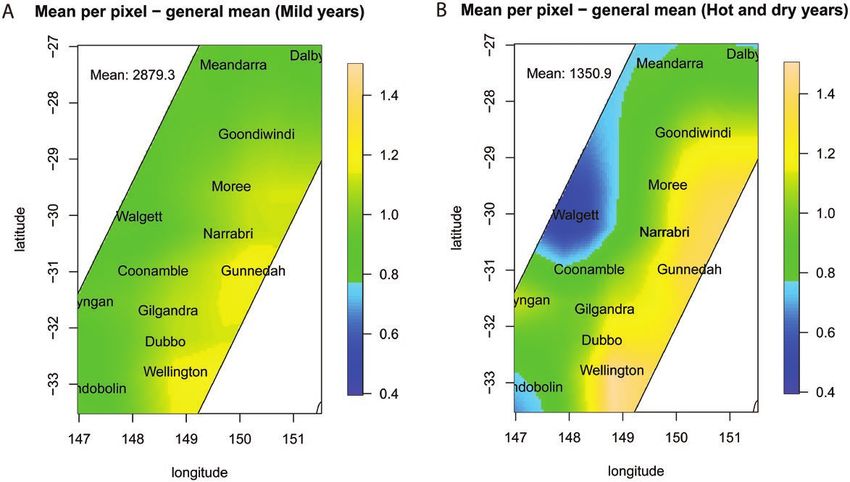
6 • Genotype-specific P-spline response surfaces
means and specific variances; Gi ∼ N(0, σg2 ), GLij ∼ N(0, σgl2 ), In model (4), yit represents the mean yield of the ith genotype in the tth
GY ik ∼ N(0, σgy2
), (GLY ijk ) ∼ N(0, σ 2 ). trial, µ stands for an intercept and Et is the fixed trial effect. The geno-
To characterize the main sources of variation and quantify the con- type main effect and the interaction are explained by M multiplicative
tribution of year types (‘s’, scenarios) to G×E variation, the model was terms. Each multiplicative term is formed by the product of a geno-
Downloaded from https://academic.oup.com/insilicoplants/article/3/2/diab018/6316219 by Wageningen University en Research -Library user on 08 October 2021
expanded to model (2): typic sensitivity bim (genotypic score) and environmental scores ztm.
Finally, εit is a residual term. To visualize how sensitivity to photoper-
y = µ + Lj + Ts + Y(T)k(s) + LYjk + GLij iod, vernalization requirements and earliness-per-se contribute to G×E,
ijk(s) 2
+ GT is + GY(T)ik(s) + GLT iks + GLY(T)ijk(s) the first two PCs estimated for G+G×E ( m=1 bim ztm in model (4))
were visualized as a GGE biplot, label-colouring genotypes according
(2) to their values for the APSIM parameters regulating phenology.
Equation (2) substitutes the random terms GY ik and GLY ijk from equa- To understand the contribution of environmental conditions to
tion (1) by the following random terms; GT is, which is the random genotypic performance, the standard GGE biplot was enriched with
interaction between genotype and year type, GY(T)ik(s) that repre- environmental information. The scaled environmental covariables
sents genotype by year (within year type) interaction, GLT iks that were regressed against the environmental PC1 and PC2 from the GGE
is the three-way genotype by location by year type interaction and model. The coefficients of these regressions were used to describe
GLY(T)ijk(s) that corresponds to a residual term that contains geno- directions of greatest change for these covariables in the biplot (Voltas
et al. 1999; Graffelman and Van Eeuwijk 2005). The direction is given
type by location by year interaction. As in model (1), all the random
by the regression coefficients and the origin. Furthermore, the angles
effects are assumed to be independent and normally distributed, with
between the direction vectors again give information about correla-
zero means and homogeneous variances. For the fixed part of the
tions: small angles between vectors mean high correlations, while
model, the year effect was partitioned into a year type (Ts ) and year
angles > 90° indicate negative correlations between the vectors.
within year type (Y(T)k(s)) effect.
As the set of genotypes used in this study was specifically segregat-
ing for APSIM parameters related to flowering time, we also assessed 2.3.3 Predicting response surfaces with P-splines embedded in a
the relative importance of those parameters, using the following model: mixed model To describe the genotypic response across latitude and
longitude, we used the following model for the APSIM yield data for
y = µ + Et + Ppd + Vrng(i) + Eps each genotype separately, i.e. conditional on i:
fgh(i)t f (i) h(i)
+ Ppd.Env + Vrn.Envg(i)t + Eps.Env Ä ät Ä ät
f (i)t h(i)t y = µ + Yk + β 1i s1 (lat)j + β 2i s2 (lon)j
ijk
+ Ppd.Vrn.Env + Ppd.Eps.Env Ä ät
fg(i)t fh(i)t
+Vrn.Eps.Env + GEfgh(i)t (3) + β 3i s3 (lat, lon)j +
ijk
gh(i)t
(5)
In model (3), yfgh(i) is the yield of genotype i in environment t (year– In equation (5), yijk is the yield of genotype i in location j and year k, Yk
location combination or trial), Et is the fixed environment effect, is the fixed year effect. The term s1 (lat)j defines the evaluation at loca-
Ppd , Vrng(i) and Eps are the random effects of the APSIM param- tion j of a set of basis functions (in vector form) for the spline fit on the
f (i) h(i)
eters that were used to generate the genotype i (see section ‘Simulated 1 t
latitude of the trial, while (β i ) is the corresponding set of genotype-
data’). These parameters regulate photoperiod response, vernalization
requirements and thermal time requirements from floral initiation to specific random coefficients (in row vector form). Similar spline terms
flowering. For the Ppd, Vrn and Eps APSIM parameters, the param-
eters defined 5, 5 and 13 classes, respectively. The interactions between are defined for longitude, (β 2 )t , and the interaction between latitude
i
APSIM parameters regulating phenology and the environment were and longitude, (β 3 )t . The interaction is orthogonal to the main effect
i
also included. The term GEfgh(i)t represents residual G×E. All random
spline terms for latitude and longitude (Wood et al. 2013; Wood 2017;
terms were assumed to be independent and normally distributed, with
zero means and homogeneous variances. Boer et al. 2020; Piepho et al. 2021). The residual term ijk contains
G×E not explained by the spline surfaces and, for real data, within trial
error. Smooth terms were fitted using first-degree P-splines with 10
2.3.2 Genotype–genotype by environment biplot To visualize the segments and first-order penalties (Eilers et al. 2015). Higher degree
contribution of APSIM parameters regulating phenology to APSIM P-splines and higher differences could also be used, but the advantage
yield and to describe their relation to genotypic performance across of using first-degree P-splines and first-order differences is that this
environments, we used a genotype–genotype by environment model model is equivalent to a linear variance model (Williams 1996; Boer
(GGE; Yan and Kang 2002; Yan and Rajcan 2002). et al. 2020). The latitude and longitude range of the spline segments
M coincides with the latitude and longitude range spanned by the trials.
y = µ + Et + bim ztm + εit The P-spline mixed model was fitted with ASReml-R v. 4 (Butler et al.
(4)
it
m=1 2017).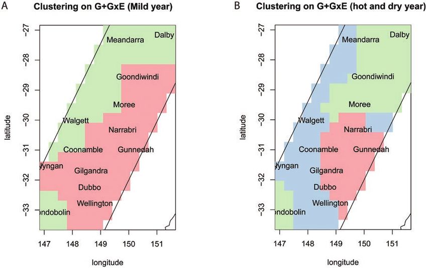
Bustos-Korts et al. • 7
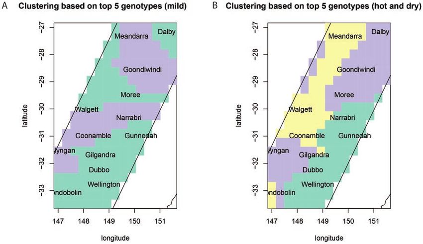
As there were contrasting year types, it made sense to predict matrix was used to calculate the Jaccard similarities between loca-
the genotypic response surfaces of each genotype across latitude tions, based on which were the five highest yielding genotypes. This
and longitude, conditional on the year type (one predicted surface similarity matrix was used for a hierarchical clustering procedure of
per genotype for ‘mild’ years and another predicted surface per gen- locations (Ward method) implemented in the ‘hclust’ function in R
Downloaded from https://academic.oup.com/insilicoplants/article/3/2/diab018/6316219 by Wageningen University en Research -Library user on 08 October 2021
otype for ‘hot and dry’ years). Then, for each genotype we used the (R Core Team 2019). The resulting regions have similar set of highest
predicted surfaces to subtract ‘mild’ years from ‘hot and dry’ years. yielding genotypes. In such a way, these regions would reflect set of
In this way, the difference in yield between ‘mild’ and ‘hot and dry’ locations for which breeders might do the same genotype selection,
years represents the sensitivity to year type, across the whole lati- at least in terms of maturity. We ran this procedure using the predic-
tude and longitude span. tions for each year type separately (i.e. producing one classification
To characterize the surfaces for explicit environmental quality, we for years with mild heat and water stress and one classification for ‘hot
fitted model (5), replacing yield as a response by the environmental and dry’ years).
indices that were used to classify years; rainfall (S2_sum.rain), aver-
age maximum temperature (S3_avg.maxt), sum of frost temperatures 2.3.4.2 Using G+G×E to cluster environments in the whole adapta-
(S2_frost.sum2) and vapour-pressure deficit (S2_vpd2) averaged tion landscape
across genotypes. Assigning locations to regions by commonality of the highest yielding
To quantify the contribution of year-to-year variation (within year genotype is a simple and straightforward method to classify locations.
type) to the total variation, we extended model (5) as follows: However, if genotypes that are in the upper yield percentiles are very
Ä ät Ä ät Ä ät similar in yield, this might lead to frequent changes in genotypic rank-
y = µ + Yk + β 1i s1 (lat)j + β 2i s2 (lon)j + β 3i s3 (lat, lon)j ing across latitude and longitude, associated to small yield differences.
ijk
Ä ät Ä ät Ä ät This potentially leads to frequent spatial discontinuities in the classi-
+ β 4ik s1 (lat)j + β 5ik s2 (lon)j + β 6ik s3 (lat, lon)j +
ijk fication of environments. A more robust procedure assigns locations
(6) to regions by the full set of fitted yields for all genotypes. Hence, we
t
created yield predictions for each genotype on a grid of 15 by 24. For
Here, the term (β 4ik ) represents the set of random coefficients for computational convenience, we reduced the grid resolution, compared
latitude (in row vector form) that are specific to each year, i.e. they are to the analysis above that looked at the winning genotype per pixel. We
scenario-dependent deviations of the genotype-specific coefficients considered that each point in the grid defined by latitude and longitude
introduced above. Similar spline terms are defined for year-by-longi- defined a (virtual) location. In this part of the analysis, each pixel cov-
ered about 28 by 28 km.
tude variation, (β 5 )t , and the contribution of year-to-year variation As in the GGE model (Yan and Kang 2002), we fitted a principal
ik
6 t components models to the genotype by virtual location matrix of
to the interaction between latitude and longitude, (β ik ) . We quanti-
the environment-centred predicted yields from the two-dimensional
fied the contribution of each model term by starting with a null model spline surfaces across years within each year type. As the first two prin-
with only a fixed year main effect. Then, we sequentially added terms cipal components explained most of the relevant variation (87.1 and
in model (6). We quantified the contribution of each term by calculat- 87.6 % for ‘mild’ and ‘hot’ years, respectively), we retained the scores
ing the difference in the residual variance between the null model and of both of them to construct a location by location similarity matrix
the model with spline terms, divided by the residual variance of the (Euclidean distances). This similarity matrix was used for a hierarchi-
null model. cal clustering procedure of locations (Ward method) implemented in
the ‘hclust’ function in R (R Core Team 2019). For each year type, the
2.3.4 Finding patterns across the genotypic response surfaces—loca- clustering procedure resulted in location classes (regions).
tion classification
2.3.4.1 Highest yielding genotypes across latitude and longitude 2.3.5 Quantifying the contribution of sensitivity to photoperiod, vernal-
We used model (5) to make predictions for each genotype over a ization requirements and earliness-per-se to the predicted adaptation
grid of 140 by 100 points that covered a latitude range from −27°S to landscape per year type The contribution of sensitivity to photoperiod,
−33.5°S and a longitude range of 147°E to 151.5°E (these ranges cor- vernalization requirements and earliness-per-se to the predicted adapta-
responded to the latitude and longitude ranges for the locations used tion surface was also quantified with a mixed model that was fitted to
in the simulations; Fig. 2). The covered area approximately spans 677 the spline-predicted yield across virtual locations. The following mixed
km from North to South and 445 km from East to West, making each model was fitted to predictions made for each year type separately, where
pixel equivalent to about 4.8 by 4.8 km. the subscript r refers to the region as identified within year type by cluster-
For each pixel on this grid (=location), we identified the five geno- ing on G+G×E of the predicted adaptation landscape;
types that had the highest yield in the tested conditions (i.e. 1 sowing
date, 1 soil condition), as predicted by the two-dimensional spline y = µ + Lj + Ppd + Vrng(i) + Eps
fgh(i) j(r) f (i) h(i)
surfaces across years within year type. The location by genotype + Ppd.Region + Vrn.Region + Eps.Region
f (i)r g(i)r h(i)r
matrix contained a 1 if a genotype was in the top five of the genotypic +Ppd.Vrn.Region + Ppd.Eps.Region
fg(i)r fh(i)r
ranking at a particular location and a 0 if it was not. This is equivalent +Vrn.Eps.Region + GEfgh(i) j(r)
to applying a selection intensity of 3.2 %. This presence or absence gh(i)r (7)
8   •   Genotype-specific P-spline response surfaces

Model (7) follows the logic of model (3), yifghr is the APSIM yield         rainfall (S2_sum.rain; Fig. 4A and B), lower maximum temperature
of the flowering time parameter combinations f, g, h, i in location j,      (S3_avg.maxt; Fig. 4C and D) and vapour-pressure deficit (S2_vpd;
Lj is the fixed location effect, Ppd , Vrng(i) and Eps are the ran-         Fig. 4E and F) than the other locations. Although the spatial pattern
                                     f (i)             h(i)
                                                                            for S3_avg.maxt2 and S2_vpd was preserved across year types, the
dom main effects of the APSIM parameters regulating photoperiod

                                                                                                                                                          Downloaded from https://academic.oup.com/insilicoplants/article/3/2/diab018/6316219 by Wageningen University en Research -Library user on 08 October 2021
                                                                            absolute values were very different between year types; ‘hot and dry’
response, vernalization requirements and thermal time requirement
                                                                            years had lower S2_sum.rain, higher S3_avg.maxt and S2_vpd than
from floral initiation to flowering (with parameters fitted as factors),
                                                                            ‘mild’ years. The spatial pattern of S2_frost.sum differed between year
nested within genotype i. The interactions between APSIM param-
                                                                            types; in ‘mild’ years, S2_frost.sum was larger in Southern locations
eters regulating phenology and regions were also included. The term
GEfgh(i) j(r) represents residual G×E.                                      than in the rest of the region, reflecting lower frost stress (Fig. 4G).
                                                                            In contrast, frost temperatures were more important in ‘hot and dry’
                                                                            years (Fig. 4H).
                          3. R E S U LTS
                     3.1 Year classification                                        3.2 Variation in flowering time and yield
The clustering procedure on environment covariables suggested two           The variation in sensitivity to photoperiod, vernalization require-
clearly defined groups of years (Fig. 3), which were contrasting in their   ments and earliness-per-se led to large variation in flowering time [see
levels of water and temperature stress. Year type 1 was characterized by    Supporting Information—Fig. 5]. Locations differed in the means
larger rainfall (S2_sum.rain; see Supporting Information—Fig. 1),           and range of days to flowering. The shortest mean duration between
lower average maximum temperature (S3_avg.maxt; see Supporting              sowing and flowering was observed in Goondiwindi, with a long-
Information—Fig. 2), less accumulation of frost temperatures (S2_           term mean across genotypes of 107 days. The largest duration was
frost.sum; see Supporting Information—Fig. 3) and lower vapour-             in Wellington, with a long-term mean across genotypes of 156 days.
pressure deficit (S2_vpd; see Supporting Information—Figs 1–4)              Within location, days to flowering did not seem to vary much between
than type 2 years. Given these differences, year type 1 can be inter-       year types [see Supporting Information—Fig. 6]. Note that the
preted as years with mild temperature and water stress (hereafter           majority of the flowering dates (25 and 75 percentiles) coincide with
referred to as ‘mild’ years), and year type 2 as years with strong tem-     the flowering ranges observed in real breeding trials. However, the
perature (heat and frost) and water stress (hereafter referred to as ‘hot   full range of flowering dates is ca. 10–25 days greater than in most
and dry’ years). Noteworthy, the relative frequency of ‘hot and dry’        breeding trials.
years has greatly increased in the most recent decades. For example,             The influence of year types was much larger on yield than on days
2 and 4 years were classified as ‘hot and dry’ in the decades 1978–87       to flowering, where year types had a strong effect on genotypic perfor-
and 1988–97, whereas 6 and 7 years were classified as ‘hot and dry’ in      mance, with ‘hot and dry’ years having in general lower yield across
the periods 1998–2007 and 2008–16 (Fig. 5). This is consistent with         locations than ‘mild’ years (Fig. 5), consistent with differences in envi-
the estimates of a trend increase of average temperature for August to      ronment quality. Given that ‘hot and dry’ years have increased in their
November of about 0.05 °C per year from 1985 to 2017 in this region         frequency during the most recent years (Fig. 5), a strategy to select for
(Fig. 3 in Ababaei and Chenu 2020).                                         wheat varieties that are well-adapted to future climate conditions could
    Within year type, there was also spatial variation for the environ-     be to select for varieties with adapted ‘flowering genetics’ or sow earlier
mental conditions (Fig. 4). Locations in the North and East had higher      (Zheng et al. 2016; Collins and Chenu 2021).

Figure 3. Cluster dendrogram to classify years based on indices S2_sum.rain, S2_frost.sum, S2_vpd and S2_avg.maxt (see details
in Table 2). Year type 1 (mild temperature and water stress) was represented by 20 years, and year type 2 (hot temperature and
strong water stress) was represented by 19 years.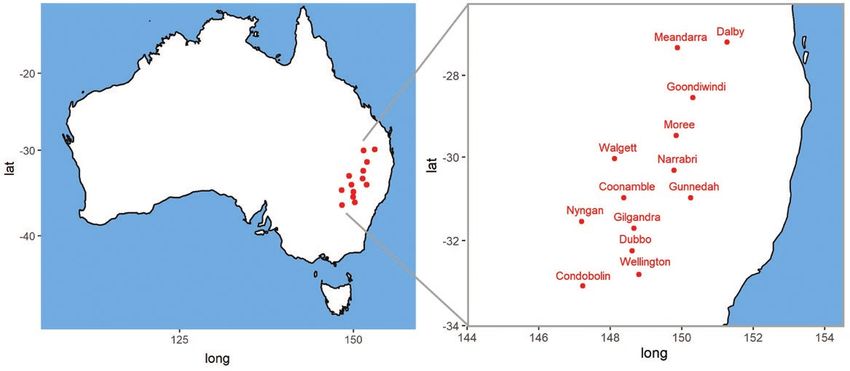
Bustos-Korts et al.   •   9

                                                                                                                                       Downloaded from https://academic.oup.com/insilicoplants/article/3/2/diab018/6316219 by Wageningen University en Research -Library user on 08 October 2021

Figure 4. (A and B) Spatial variation for rainfall (S2_sum.rain); (C and D) average maximum temperature (S3_avg.maxt); (E and
F) average vapour-pressure deficit (S2_vpd); (G and H) the sum of frost temperatures (S2_frost.sum) for ‘mild’ and ‘hot and dry’
(HD) years. The four indices were calculated in a period from flowering + 100 °Cd to flowering + 600 °Cd. Surfaces were fitted
simultaneously to the environmental indices calculated for all genotypes using model (5). Missing predictions for S2_frost.sum in
HD years indicate locations in which no frost was observed.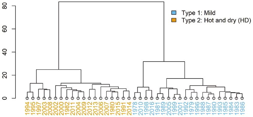
10 •      Genotype-specific P-spline response surfaces

Table 3. Variance components for the simulated yield data of                Table 5. Contribution of the APSIM traits regulating
156 genotypes over 39 years at 13 locations (in total 503 year–             phenology to yield variation. Variance components were
location combinations because four of them were removed due                 estimated by fitting the statistical model to 156 genotypes at 13
to crop failure).                                                           locations over 39 years.

                                                                                                                                                       Downloaded from https://academic.oup.com/insilicoplants/article/3/2/diab018/6316219 by Wageningen University en Research -Library user on 08 October 2021
Component                      Variance                  Standard error     Term                         Component                  Standard error
Geno                            86 559                       10 380         Ppd                            49 610                       35 182
Geno:Loc                        37 528                        1408          Vrn                             5538                         3971
Geno:Year                       60 023                        1407          Eps                            31 056                       12 783
Residual                       208 106                        1115          Ppd:env                        62 232                        2287
                                                                            Vrn:env                        25 992                        1178
                                                                            Eps:env                        97 832                        2355
                                                                            Ppd:Vrn:env                     4593                           232
Table 4. Variance components for the simulated yield data of
                                                                            Ppd:Eps:env                    69 719                          788
156 genotypes over 39 years at 13 locations (total of 503 year–
                                                                            Vrn:Eps:env                    68 178                          798
location combinations) based on genotype and genotype
                                                                            Residual                       22 221                          232
interactions with location or year type.
Component                           Variance             Standard error
                                                                             3.5 Contribution of APSIM parameters regulating
Geno                                 71 280                  10 414                       flowering time to G×E
Geno:Loc                             29 975                   1461          We also estimated the contribution of APSIM parameters regulating
Geno:Type                            28 852                   3764          flowering time on yield. Across the 503 environments considered in this
Geno:Year within Type                45 304                   1140          analysis, the largest contribution to the yield G×E was made the three-
Geno:Loc:Type                        14 965                     834         way interactions, especially Ppd:Eps:Env and Vrn:Eps:Env (Table 5).
Residual                            200 468                   1088          This implies that specific combinations of photoperiod and vernaliza-
                                                                            tion alleles, in combination with different earliness-per-se levels make
                                                                            important contributions to wheat adaptation across environments.
 3.3 Variance components for yield across locations                         The two-way interactions between Eps:Env and Ppd:Env also made
                   and years                                                very important contributions to the total G×E variation (Table 5). The
The variance components model indicates that there is large G×E             same result can be illustrated in Supporting Information—Figs 7
for yield in this data set (Table 3). Most of the G×E is not consistent     and 8 that describe the relationship between yield and flowering time
from one year to the next and is mainly related to the two-way geno-        for each of the environments. In most environments, this relationship
type by year interaction and the three-way interaction between geno-        shows an optimum, but the position of this optimum between yield
types, locations and years (captured in the residual in Table 3). For the   and days to flowering depends on the year–location combination.
two-way genotype by year interaction, we used explicit covariables to           When assessing the relationship between yield and the
classify years in groups that are more internally homogeneous and pre-      APSIM parameters regulating phenology, it can be observed
dictable. For example, from explicit covariables, as we did here and as     that for all environments there is an optimum Eps value, and that
done in Chenu et al. (2011); Zheng et al. (2018), or from long-term         the position and height of this optimum depends on the spe-
frequencies, as done in Chenu et al. (2013). The genotype by location       cific combinations of Ppd and Vrn values (Fig. 6). Furthermore,
interaction will be examined by fitting smooth surfaces with P-splines      the effect of Ppd and Vrn on yield is much larger in ‘mild’ than in
across latitude and longitudes.                                             ‘hot and dry’ years, leading to a larger phenotypic variance in
                                                                            ‘mild’ than in ‘hot and dry’ years (as already observed in Figs 4
                                                                            and 5). There is a large interaction between earliness-per-se and Ppd/
      3.4 Variance components for yield between                             Vrn values, shown in the yield crossing overs in all locations and
                     year types                                             year types. However, the optimum combination of Eps and Ppd/
Upon integrating year type in the G×E analysis (Table 4), we see that       Vrn depends on the location, and it is also highly influenced by year
the variance component for genotype by location by year type interac-       type. This explains the large and complex G×E observed in this data
tion is about half the magnitude of the variance component for geno-        set. The Eps value that leads to optimum yield is in general lower for
type by location interaction. Therefore, it will be interesting to model    hot than for ‘mild’ years, coinciding with the general observation
the genotype by location interaction by explicit functions conditional      that long-cycle genotypes run out of water in ‘hot and dry’ years. In
on the year type. Variance components for individual effects in Table 3     ‘hot and dry years’, the optimum combination of APSIM parameter
are different from those of Table 4 (especially the genotype main           values is an intermediate value of Eps with large values for Ppd and
effect) because of the absence of some locations in particular years        Vrn. However, when Eps is larger than 700 °Cd, genotypes with a
(four year–location combinations were removed because of large crop         lower value of Ppd/Vrn have an advantage. This leads to large crosso-
failure in those environments).                                             ver G×E in this data set (Fig. 6). In contrast, for any Eps value in
Bustos-Korts et al. • 11
‘mild’ years, having large Ppd and Vrn values is an advantage, com- Fig. 7, examining the relative positions of the vectors for envi-
pared to low values for Ppd and Vrn. When repeating the analysis for ronment indices and genotypic parameters regulating flowering
the periods 1978–97 and 1998–2016, earlier-flowering genotypes, time gives insight in the underlying physiological mechanisms of
determined either by lower Eps values or by higher Eps values in G×E in this data set. In ‘hot and dry’ years, Eps induced a large
Downloaded from https://academic.oup.com/insilicoplants/article/3/2/diab018/6316219 by Wageningen University en Research -Library user on 08 October 2021
combination with small values for Ppd/Vrn, are favoured in the most G×E interaction with warmer and dryer environments (this can
recent decades [see Supporting Information—Fig. 8]. be observed by the almost opposite position of the vector for Eps
A GGE analysis per year type characterized the effect of com- with S2_avg.max and S2_vpd). In Fig. 6, this can be observed as
binations of flowering time parameters on G×E for yield (Fig. the position of the optimum for yield, in relation to Eps values,
7). In both years, the genotype main effect (Geno_mean) was occurs at higher values for environments that are less drought-
more associated to larger values of Ppd (smaller angle between prone, like ‘Narrabri’ or ‘Wellington’ (Fig. 4). This indicates that
vectors), than to the Vrn and Eps. This result coincides with when more water is available, it is advantageous to have larger
Fig. 6, which showed that larger values for Ppd generally lead to values for Eps (hence, later flowering), compared to very dry
larger yields. In contrast, Eps contributed more to G×E than to environments. In ‘mild’ years, Eps also had a positive interac-
the genotype main effect. These results coincide with the vari- tion with more favourable environments that had a larger rainfall
ance components model in Table 5 and with Fig. 6, which shows (S2_sum.rain2). Larger values for Ppd and Vrn contributed to
that the optimum value for Eps depends on the environment. In generate a negative interaction with warmer environments (i.e.
Figure 5. Variation in APSIM-simulated yield (kg ha−1) associated to locations, years and year type. ‘Hot and dry’ (HD)
environments correspond to years with high temperature and water stress, whereas ‘mild’ environments correspond to years with
mild temperature and water stress.12 • Genotype-specific P-spline response surfaces
A P pd , mild years
Goondiwindi Moree Narrabri Gunnedah Coonamble Gilgandra Nyngan Dalby Meandarra Walgett Condobolin Dubbo Wellington
4000
P pd
Downloaded from https://academic.oup.com/insilicoplants/article/3/2/diab018/6316219 by Wageningen University en Research -Library user on 08 October 2021
3000
Yield (kg/ha)
0
0.3
2000 0.6
0.9
1000 1.2
40 0
40 0
40 0
40 0
40 0
40 0
40 0
40 0
40 0
40 0
40 0
40 0
00
0
0
0
0
0
0
0
0
0
0
0
0
0
0
0
0
0
0
0
0
0
0
0
0
0
0
0
0
0
0
0
0
0
0
0
0
0
0
0
0
0
0
0
0
0
0
0
0
0
0
0
40
60
80
60
80
60
80
60
80
60
80
60
80
60
80
60
80
60
80
60
80
60
80
60
80
60
80
10
10
10
10
10
10
10
10
10
10
10
10
10
Earliness − per − se
B P pd , hot and dry years
Goondiwindi Moree Narrabri Gunnedah Coonamble Gilgandra Nyngan Dalby Meandarra Walgett Condobolin Dubbo Wellington
P pd
2000
Yield (kg/ha)
0
0.3
0.6
1000
0.9
1.2
0
40 0
40 0
40 0
40 0
40 0
40 0
40 0
40 0
40 0
40 0
40 0
40 0
00
0
0
0
0
0
0
0
0
0
0
0
0
0
0
0
0
0
0
0
0
0
0
0
0
0
0
0
0
0
0
0
0
0
0
0
0
0
0
0
0
0
0
0
0
0
0
0
0
0
0
0
40
60
80
60
80
60
80
60
80
60
80
60
80
60
80
60
80
60
80
60
80
60
80
60
80
60
80
10
10
10
10
10
10
10
10
10
10
10
10
10
Earliness − per − se
C V rn, mild years
Goondiwindi Moree Narrabri Gunnedah Coonamble Gilgandra Nyngan Dalby Meandarra Walgett Condobolin Dubbo Wellington
4000
V rn
Yield (kg/ha)
0.9
3000 1.1
1.3
2000 1.5
1.7
1000
40 0
40 0
40 0
40 0
40 0
40 0
40 0
40 0
40 0
40 0
40 0
40 0
00
0
0
0
0
0
0
0
0
0
0
0
0
0
0
0
0
0
0
0
0
0
0
0
0
0
0
0
0
0
0
0
0
0
0
0
0
0
0
0
0
0
0
0
0
0
0
0
0
0
0
0
40
60
80
60
80
60
80
60
80
60
80
60
80
60
80
60
80
60
80
60
80
60
80
60
80
60
80
10
10
10
10
10
10
10
10
10
10
10
10
10
Earliness − per − se
D V rn, hot and dry years
Goondiwindi Moree Narrabri Gunnedah Coonamble Gilgandra Nyngan Dalby Meandarra Walgett Condobolin Dubbo Wellington
3000
V rn
Yield (kg/ha)
0.9
2000 1.1
1.3
1.5
1000
1.7
40 0
40 0
40 0
40 0
40 0
40 0
40 0
40 0
40 0
40 0
40 0
40 0
00
0
0
0
0
0
0
0
0
0
0
0
0
0
0
0
0
0
0
0
0
0
0
0
0
0
0
0
0
0
0
0
0
0
0
0
0
0
0
0
0
0
0
0
0
0
0
0
0
0
0
0
40
60
80
60
80
60
80
60
80
60
80
60
80
60
80
60
80
60
80
60
80
60
80
60
80
60
80
10
10
10
10
10
10
10
10
10
10
10
10
10
Earliness − per − se
Figure 6. APSIM-simulated yield for genotypes as function of the values for the APSIM parameters earliness-per-se (Eps) and
sensitivity to photoperiod (Ppd, A and B) or vernalization (Vrn, C and D), in ‘mild’ at ‘hot and dry’ (HD) years. Colours of the
facet headers correspond to the regions within year types as shown in Fig. 11.
those with larger values for S2_avg.max). In Fig. 6, this can, 3.6 Spline surfaces across latitude and longitude for
for example, be observed as lower Ppd and Vrn values leading each year type
to a larger yield in drought-prone locations like ‘Meandarra’, As the interaction of genotype and year type was large (Table 4 and
‘Goondiwindi’ and ‘Dalby’ (Fig. 4). GT is in equation (2)), it is potentially useful to inspect the spline-fittedBustos-Korts et al. • 13
Downloaded from https://academic.oup.com/insilicoplants/article/3/2/diab018/6316219 by Wageningen University en Research -Library user on 08 October 2021
Figure 7. Genotype–genotype by environment (GGE) biplot for APSIM yield in ‘mild’ and ‘hot and dry’ years. Colour dots
indicate the APSIM parameter values for sensitivity to photoperiod (Ppd, A and B), vernalization requirement (Vrn, C and D)
and thermal time from floral initiation to flowering (earliness-per-se; Eps, E and F). Black vectors indicate the direction of greatest
change of environmental covariables and the environment means for grain yield (Env_means). Red vectors indicate the direction
of greatest change in the APSIM parameters regulating flowering time and genotype means for grain yield (Geno_mean_yld) and
days to heading (Geno_mean_heading) across environments.14 • Genotype-specific P-spline response surfaces
surfaces per year type. We quantified the contribution of each term in In contrast, in ‘hot and dry’ years, the best locations had average yields
the P-spline model by sequentially adding those terms and comput- that were about 1.5 times the general mean (i.e. still lower than mean
ing the reduction in the residual after including an additional model yield in a mild year) and the poorest locations had average yields that
term (equation (6); see Supporting Information—Fig. 9). The were about 0.4 times the general mean, i.e. the gradient of environmen-
Downloaded from https://academic.oup.com/insilicoplants/article/3/2/diab018/6316219 by Wageningen University en Research -Library user on 08 October 2021
relative importance of latitude, longitude, their two-way interactions tal quality was much stronger in ‘hot and dry’ than in ‘mild’ years. This
and their three-way interactions with year indicate that ‘hot and dry’ coincides with Fig. 8A, which show a larger difference in phenotypic
years in general required a larger model complexity, as the interactions variances in more rainy places in ‘mild’ years.
between latitude and longitude with year explained a larger propor- Besides inspecting the gradients in average yield per year type, we
tion of the variation than in ‘mild’ years. In ‘hot and dry’ years, geno- examined the response surfaces for individual genotypes and focused
types also differed more in the contribution of each model term [see on the yield difference between ‘hot and dry’ and ‘mild’ years across
Supporting Information—Fig. 9]. latitude and longitude for each genotype (Fig. 9). Most genotypes
When inspecting the predicted response surfaces for each geno- showed a large yield reduction when comparing ‘hot and dry’ and ‘mild’
type and year type, ‘mild’ years had an average yield that was 2.13 years. Only few of them (e.g. ‘g0_0.9_425’; Fig. 9A) had a similar yield
times larger than that of ‘hot and dry’ years (2879 vs. 1351 kg ha−1; (or even larger yield for some locations) in ‘hot and dry’ than in ‘mild’
Fig. 8). For both ‘mild’ and ‘hot and dry’ years, there was a yield gradi- years, causing strong G×E within and between year types (Fig. 9A).
ent; average yield per virtual location (pixel) was larger in the East and These exceptional genotypes were very early flowering, with small val-
South-East (close to locations Wellington and Gunnedah), than in the ues for the three flowering time parameters and a very low mean yield
West (especially in locations Walgett and Meandarra). This aligns with (e.g. mean yield of ‘g0_0.9_425’ in mild years was 773.9 kg ha−1; Fig.
the rainfall isohyets which decrease from NW to SE in this part of the 9A). Genotypes with small Eps values, but larger sensitivity to pho-
country (Chenu et al. 2011). toperiod (e.g. ‘g1.2_0.9_425’; Fig. 9B) had much larger average yield
However, the average yield deviation for each virtual location than ‘g0_0.9_425’ (2053.5 vs. 773.9 kg ha−1 in mild years; Fig. 9A) and
(pixel) in the latitude–longitude range spanned by the trials, compared showed an intermediate behaviour; maintaining or increasing yield
to the mean yield, was much less in ‘mild’ than in ‘hot and dry’ years. in ‘hot and dry’ compared to ‘mild’ years in South-Eastern locations,
In ‘mild’ years, the best locations had average yields that were about 1.3 and reducing yield in Western locations, in ‘hot and dry’ compared to
times the general mean (for the same year type), and the worst loca- ‘mild’ years (Fig. 9). The locations that led to a yield increase in ‘hot
tions had average yields that were about 0.8 times the general mean. and dry’ years for genotypes similar to ‘g0_0.9_425’ (Fig. 9A) were
Figure 8. For ‘mild’ years (A) and ‘hot and dry’ years (B), ratio between the mean predicted yield at each pixel in the whole
latitude and longitude range spanned by the trial locations (calculated across the 156 genotypes and years within year type), and
the general mean (calculated across all genotypes, pixels and years within year type).You can also read