Hard negative examples are hard, but useful
←
→
Page content transcription
If your browser does not render page correctly, please read the page content below
Hard negative examples are hard, but useful

                                         Hong Xuan1[0000−0002−4951−3363], Abby Stylianou2, Xiaotong Liu1, and Robert Pless1
                                                       1
                                                           The George Washington University, Washington DC 20052
                                                               {xuanhong,liuxiaotong2017,pless}@gwu.edu
                                                               2
                                                                 Saint Louis University, St. Louis MO 63103
                                                                        abby.stylianou@slu.edu
arXiv:2007.12749v1 [cs.CV] 24 Jul 2020

                                                Abstract. Triplet loss is an extremely common approach to distance metric
                                                learning. Representations of images from the same class are optimized to be
                                                mapped closer together in an embedding space than representations of images
                                                from different classes. Much work on triplet losses focuses on selecting the
                                                most useful triplets of images to consider, with strategies that select dissimilar
                                                examples from the same class or similar examples from different classes. The
                                                consensus of previous research is that optimizing with the hardest negative
                                                examples leads to bad training behavior. That’s a problem – these hardest neg-
                                                atives are literally the cases where the distance metric fails to capture semantic
                                                similarity. In this paper, we characterize the space of triplets and derive why
                                                hard negatives make triplet loss training fail. We offer a simple fix to the loss
                                                function and show that, with this fix, optimizing with hard negative examples
                                                becomes feasible. This leads to more generalizable features, and image retrieval
                                                results that outperform state of the art for datasets with high intra-class vari-
                                                ance. Code is available at: https://github.com/littleredxh/HardNegative.git

                                                Keywords: Hard Negative, Deep Metric Learning, Triplet Loss

                                         1   Introduction

                                         Deep metric learning optimizes an embedding function that maps semantically sim-
                                         ilar images to relatively nearby locations and maps semantically dissimilar images
                                         to distant locations. A number of approaches have been proposed for this prob-
                                         lem [4,9,12,16,17,18,26]. One common way to learn the mapping is to define a loss
                                         function based on triplets of images: an anchor image, a positive image from the same
                                         class, and a negative image from a different class. The loss penalizes cases where the
                                         anchor is mapped closer to the negative image than it is to the positive image.
                                             In practice, the performance of triplet loss is highly dependent on the triplet
                                         selection strategy. A large number of triplets are possible, but for a large part of the
                                         optimization, most triplet candidates already have the anchor much closer to the
                                         positive than the negative, so they are redundant. Triplet mining refers to the process
                                         of finding useful triplets.
                                             Inspiration comes from Neil DeGrasse Tyson, the famous American Astrophysicist
                                         and science educator who says, while encouraging students, “In whatever you choose to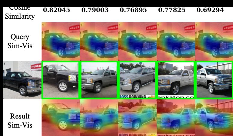
2 H. Xuan et al.
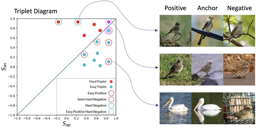
Fig. 1: The triplet diagram plots a triplet as a dot defined by the anchor-positive
similarity Sap on the x-axis and the anchor-negative similarity San on the y-axis. Dots
below the diagonal correspond to triplets that are “correct”, in the sense that the same
class example is closer than the different class example. Triplets above the diagonal of
the diagram are candidates for the hard negative triplets. They are important because
they indicate locations where the semantic mapping is not yet correct. However,
previous works have typically avoided these triplets because of optimization challenges.
do, do it because it is hard, not because it is easy”. Directly mapping this to our case sug-
gests hard negative mining, where triplets include an anchor image where the positive
image from the same class is less similar than the negative image from a different class.
Optimizing for hard negative triplets is consistent with the actual use of the
network in image retrieval (in fact, hard negative triplets are essentially errors in the
trained image mappings), and considering challenging combinations of images has
proven critical in triplet based distance metric learning [4,6,8,16,21]. But challenges
in optimizing with the hardest negative examples are widely reported in work on
deep metric learning for face recognition, people re-identification and fine-grained
visual recognition tasks. A variety of work shows that optimizing with the hardest
negative examples for deep metric learning leads to bad local minima in the early
phase of the optimization [27,2,16,22,28,18,3].
A standard version of deep metric learning uses triplet loss as the optimization
function to learn the weights of a CNN to map images to a feature vector. Very
commonly, these feature vectors are normalized before computing the similarity
because this makes comparison intuitive and efficient, allowing the similarity between
feature vectors to be computed as a simple dot-product. We consider this network to
project points to the hypersphere (even though that projection only happens during
the similarity computation). We show there are two problems in this implementation.
First, when the gradient of the loss function does not consider the normalization
to a hypersphere during the gradient backward propagation, a large part of the
gradient is lost when points are re-projected back to the sphere, especially in the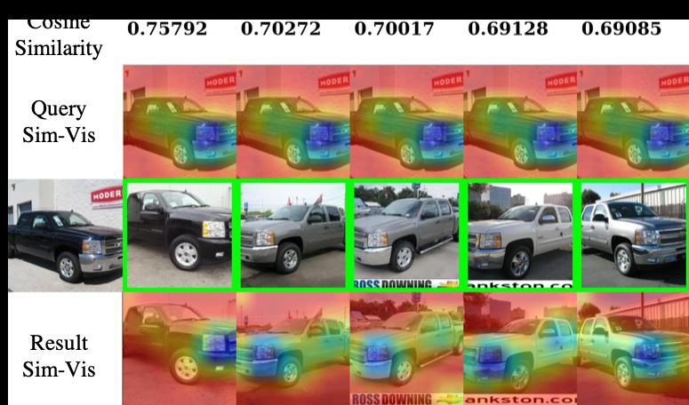
Hard negative examples are hard, but useful       3

cases of triplets including nearby points. Second, when optimizing the parameters
(the weights) of the network for images from different classes that are already mapped
to similar feature points, the gradient of the loss function may actually pull these
points together instead of separating them (the opposite of the desired behavior).
    We give a systematic derivation showing when and where these challenging triplets
arise and diagram the sets of triplets where standard gradient descent leads to bad
local minima, and do a simple modification to the triplet loss function to avoid bad
optimization outcomes.
    Briefly, our main contributions are to:
 – introduce the triplet diagram as a visualization to help systematically characterize
   triplet selection strategies,
 – understand optimization failures through analysis of the triplet diagram,
 – propose a simple modification to a standard loss function to fix bad optimization
   behavior with hard negative examples, and
 – demonstrate this modification improves current state of the art results on datasets
   with high intra-class variance.

2    Background
Triplet loss approaches penalize the relative similarities of three examples – two from
the same class, and a third from a different class. There has been significant effort
in the deep metric learning literature to understand the most effective sampling of
informative triplets during training. Including challenging examples from different
classes (ones that are similar to the anchor image) is an important technique to speed
up the convergence rate, and improve the clustering performance. Currently, many
works are devoted to finding such challenging examples within datasets. Hierarchical
triplet loss (HTL) [4] seeks informative triplets based on a pre-defined hierarchy of
which classes may be similar. There are also stochastic approaches [21] that sample
triplets judged to be informative based on approximate class signatures that can be
efficiently updated during training.
     However, in practice, current approaches cannot focus on the hardest negative
examples, as they lead to bad local minima early on in training as reported in
[27,16,2,3,18,22,28]. The avoid this, authors have developed alternative approaches,
such as semi-hard triplet mining [16], which focuses on triplets with negative examples
that are almost as close to the anchor as positive examples. Easy positive mining [27]
selects only the closest anchor-positive pairs and ensures that they are closer than
nearby negative examples.
     Avoiding triplets with hard negative examples remedies the problem that the
optimization often fails for these triplets. But hard negative examples are important.
The hardest negative examples are literally the cases where the distance metric fails
to capture semantic similarity, and would return nearest neighbors of the incorrect
class. Interesting datasets like CUB [24] and CAR [10] which focus on birds and cars,
respectively, have high intra-class variance – often similar to or even larger than the
inter-class variance. For example, two images of the same species in different lighting
and different viewpoints may look quite different. And two images of different bird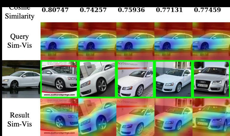
4         H. Xuan et al.

species on similar branches in front of similar backgrounds may look quite similar.
These hard negative examples are the most important examples for the network to
learn discriminative features, and approaches that avoid these examples because of
optimization challenges may never achieve optimal performance.
    There has been other attention on ensure that the embedding is more spread
out. A non-parametric approach [25] treats each image as a distinct class of its own,
and trains a classifier to distinguish between individual images in order to spread
feature points across the whole embedding space. In [29], the authors proposed a
spread out regularization to let local feature descriptors fully utilize the expressive
power of the space. The easy positive approach [27] only optimizes examples that are
similar, leading to more spread out features and feature representations that seem
to generalize better to unseen data.
    The next section introduces a diagram to systematically organize these triplet
selection approaches, and to explore why the hardest negative examples lead to bad
local minima.

3      Triplet diagram
Triplet loss is trained with triplets of images, (xa,xp,xn), where xa is an anchor
image, xp is a positive image of the same class as the anchor, and xn is a negative
image of a different class. We consider a convolution neural network, f(·), that
embeds the images on a unit hypersphere, (f(xa),f(xp),f(xn)). We use (fa,fp,fn) to
simplify the representation of the normalized feature vectors. When embedded on
a hypersphere, the cosine similarity is a convenient metric to measure the similarity
between anchor-positive pair Sap = fa|fp and anchor-negative pair San = fa|fn, and
this similarity is bounded in the range [−1,1].
    The triplet diagram is an approach to characterizing a given set of triplets. Figure 1
represents each triplet as a 2D dot (Sap,San), describing how similar the positive and
negative examples are to the anchor. This diagram is useful because the location on
the diagram describes important features of the triplet:
    – Hard triplets: Triplets that are not in the correct configuration, where the
      anchor-positive similarity is less than the anchor-negative similarity (dots above
      the San = Sap diagonal). Dots representing triplets in the wrong configuration
      are drawn in red. Triplets that are not hard triplets we call Easy Triplets, and
      are drawn in blue.
    – Hard negative mining: A triplet selection strategy that seeks hard triplets, by
      selecting for an anchor, the most similar negative example. They are on the top
      of the diagram. We circle these red dots with a blue ring and call them hard
      negative triplets in the following discussion.
    – Semi-hard negative mining[16]: A triplet selection strategy that selects, for
      an anchor, the most similar negative example which is less similar than the
      corresponding positive example. In all cases, they are under San =Sap diagonal.
      We circle these blue dots with a red dashed ring.
    – Easy positive mining[27]: A triplet selection strategy that selects, for an an-
      chor, the most similar positive example. They tend to be on the right side of the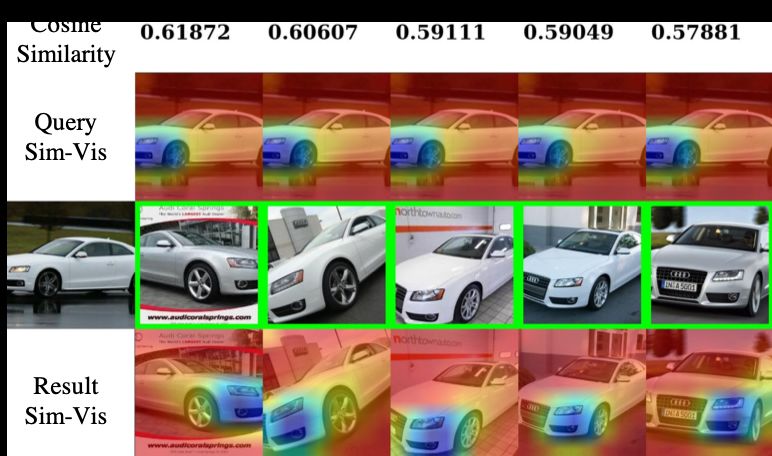
Hard negative examples are hard, but useful       5

   diagram because the anchor-positive similarity tends to be close to 1. We circle
   these blue dots with a red ring.
 – Easy positive, Hard negative mining[27]: A related triplet selection strategy
   that selects, for an anchor, the most similar positive example and most similar
   negative example. The pink dot surrounded by a blue dashed circle represents
   one such example.

4    Why some triplets are hard to optimize
The triplet diagram offers the ability to understand when the gradient-based opti-
mization of the network parameters is effective and when it fails. The triplets are
used to train a network whose loss function encourages the anchor to be more similar
to its positive example (drawn from the same class) than to its negative example
(drawn from a different class). While there are several possible choices, we consider
NCA [5] as the loss function:
                                               exp(Sap)
                       L(Sap,San)=−log                                             (1)
                                          exp(Sap)+exp(San)
   All of the following derivations can also be done for the margin-based triplet loss
formulation used in [16]. We use the NCA-based of triplet loss because the following
gradient derivation is clear and simple. Analysis of the margin-based loss is similar
and is derived in the Appendix.
   The gradient of this NCA-based triplet loss L(Sap,San) can be decomposed into
two parts: a single gradient with respect to feature vectors fa, fp, fn:

               ∂L ∂Sap   ∂L ∂San         ∂L ∂Sap        ∂L ∂San
       ∆L=(            +         )∆fa +          ∆fp +          ∆fn                (2)
              ∂Sap ∂fa ∂San ∂fa         ∂Sap ∂fp       ∂San ∂fn
  and subsequently being clear that these feature vectors respond to changes in the
model parameters (the CNN network weights), θ:

           ∂L ∂Sap       ∂L ∂San ∂fa           ∂L ∂Sap ∂fp          ∂L ∂San ∂fn
    ∆L=(              +            )     ∆θ+                 ∆θ+                  ∆θ
          ∂Sap ∂fa ∂San ∂fa ∂θ                ∂Sap ∂fp ∂θ          ∂San ∂fn ∂θ
                                                                                    (3)
    The gradient optimization only affects the feature embedding through variations
in θ, but we first highlight problems with hypersphere embedding assuming that the
optimization could directly affect the embedding locations without considering the
gradient effect caused by θ. To do this, we derive the loss gradient, ga, gp, gn, with
respect to the feature vectors, fa, fp, fn, and use this gradient to update the feature
locations where the error should decrease:
                                                ∂L
                      fpnew =fp −αgp =fp −α         =fp +βfa                        (4)
                                                ∂fp
                                                ∂L
                      fnnew =fn −αgn =fn −α         =fn −βfa                        (5)
                                                ∂fn
                                                ∂L
                      fanew =fa −αga =fa −α         =fa −βfn +βfp                   (6)
                                                ∂fa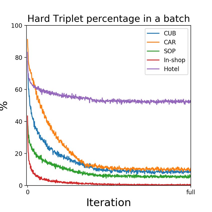
6       H. Xuan et al.

where β =α exp(Sexp(S an )
                 ap )+exp(San )
                                and α is the learning rate.
    This gradient update has a clear geometric meaning: the positive point fp is encour-
aged to move along the direction of the vector fa; the negative point fn is encouraged
to move along the opposite direction of the vector fa; the anchor point fa is encouraged
to move along the direction of the sum of fp and −fn. All of these are weighted by
the same weighting factor β. Then we can get the new anchor-positive similarity and
anchor-negative similarity (the complete derivation is given in the Appendix):
                          new
                         Sap  =(1+β 2)Sap +2β−βSpn −β 2San                           (7)
                          new
                         San  =(1+β 2)San −2β+βSpn −β 2Sap                           (8)

    The first problem is these gradients, ga, gp, gn, have components that move
them off the sphere; computing the cosine similarity requires that we compute the
norm of fanew , fpnew and fnnew (the derivation for these is shown in Appendix).
Given the norm of the updated feature vector, we can calculate the similarity change
after the gradient update:
                                           Snew
                             ∆Sap = kfa newap
                                           kkfp new k −Sap                           (9)
                                          Snew
                                           kkfn new k −San
                             ∆San = kfa newan                                       (10)

     Figure 2(left column) shows calculations of the change in the anchor-positive simi-
larity and the change in the anchor-negative similarity. There is an area along the right
side of the ∆Sap plot (top row, left column) highlighting locations where the anchor
and positive are not strongly pulled together. There is also a region along the top side
of the ∆San plot (bottom row, left column) highlighting locations where the anchor
and negative can not be strongly separated. This behavior arises because the gradient
is pushing the feature off the hypersphere and therefore, after normalization, the effect
is lost when anchor-positive pairs or anchor-negative pairs are close to each other.
     The second problem is that the optimization can only control the feature
vectors based on the network parameters, θ. Changes to θ are likely to affect nearby
points in similar ways. For example, if there is a hard negative triplet, as defined in
Section 3, where the anchor is very close to a negative example, then changing θ to
move the anchor closer to the positive example is likely to pull the negative example
along with it. We call this effect “entanglement” and propose a simple model to
capture its effect on how the gradient update affects the similarities.
     We use a scalar, p, and a similarity related factor q = SapSan, to quantify this
entanglement effect. When all three examples in a triplet are nearby to each other,
both Sap and San will be large, and therefore q will increase the entanglement effect;
when either the positive or the negative example is far away from the anchor, one
of Sap and San will be small and q will reduce the entanglement effect.
     The total similarity changes with entanglement will be modeled as follows:
                                total
                              ∆Sap    =∆Sap +pq∆San                                 (11)
                                total
                              ∆San      =∆San +pq∆Sap                               (12)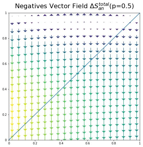
Hard negative examples are hard, but useful        7

Fig. 2: Numerical simulation of how the optimization changes triplets, with 0
entanglement (left), some entanglement (middle) and complete entanglement (right).
The top row shows effects on anchor-positive similarity the bottom row shows effects
on anchor-negative similarity. The scale of the arrows indicates the gradient strength.
The top region of the bottom-middle and bottom-right plots highlight that the hard
negative triplets regions are not well optimized with standard triplet loss.

    Figure 2(middle and right column) shows vector fields on the diagram where Sap
and San will move based on the gradient of their loss function. It highlights the region
along right side of the plots where that anchor and positive examples become less
             total
similar (∆Sap      < 0), and the region along top side of the plots where that anchor
                                                     total
and negative examples become more similar (∆San            > 0) for different parameters
of the entanglement.
    When the entanglement increases, the problem gets worse; more anchor-negative
pairs are in a region where they are pushed to be more similar, and more anchor-
positive pairs are in a region where they are pushed to be less similar. The anchor-
positive behavior is less problematic because the effect stops while the triplet is still
in a good configuration (with the positive closer to the anchor than the negative),
while the anchor-negative has not limit and pushes the anchor and negative to be
completely similar.
    The plots predict the potential movement for triplets on the triplet diagram. We
will verify this prediction in the Section 6.

Local minima caused by hard negative triplets In Figure 2, the top region
indicates that hard negative triplets with very high anchor-negative similarity get
pushed towards (1,1). Because, in that region, San will move upward to 1 and Sap will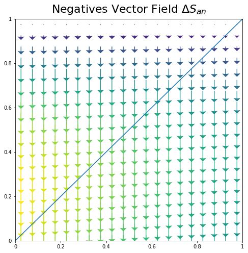
8       H. Xuan et al.

move right to 1. The result of the motion is that a network cannot effectively separate
the anchor-negative pairs and instead pushes all features together. This problem was
described in [27,16,2,3,18,22,28] as bad local minima of the optimization.

When will hard triplets appear During triplet loss training, a mini-batch of
images is samples random examples from numerous classes. This means that for every
image in a batch, there are many possible negative examples, but a smaller number
of possible positive examples. In datasets with low intra-class variance and high
inter-class variance, an anchor image is less likely to be more similar to its hardest
negative example than its random positive example, resulting in more easy triplets.
    However, in datasets with relatively higher intra-class variance and lower inter-class
variance, an anchor image is more likely to be more similar to its hardest negative
example than its random positive example, and form hard triplets. Even after several
epochs of training, it’s difficult to cluster instances from same class with extremely
high intra-class variance tightly.

5    Modification to triplet loss

Our solution for the challenge with hard negative triplets is to decouple them into
anchor-positive pairs and anchor-negative pairs, and ignore the anchor-positive pairs,
and introduce a contrastive loss that penalizes the anchor-negative similarity. We call
this Selectively Contrastive Triplet loss LSC , and define this as follows:
                                     (
                                       λSan          if San >Sap
                    LSC (Sap,San)=                                                (13)
                                       L(Sap,San) others

    In most triplet loss training, anchor-positive pairs from the same class will be
always pulled to be tightly clustered. With our new loss function, the anchor-positive
pairs in triplets will not be updated, resulting in less tight clusters for a class of
instances (we discuss later how this results in more generalizable features that are
less over-fit to the training data). The network can then ‘focus’ on directly pushing
apart the hard negative examples.
    We denote triplet loss with a Hard Negative mining strategy (HN), triplet loss
trained with Semi-Hard Negative mining strategy (SHN), and our Selectively Con-
trastive Triplet loss with hard negative mining strategy (SCT) in the following
discussion.
    Figure 3 shows four examples of triplets from the CUB200(CUB) [24] and
CAR196(CAR) [10] datasets at the very start of training, and Figure 4 shows four
examples of triplets at the end of training. The CUB dataset consists of various
classes of birds, while the CAR196 dataset consists of different classes of cars. In
both of the example triplet figures, the left column shows a positive example, the
second column shows the anchor image, and then we show the hard negative example
selected with SCT and SHN approach.
    At the beginning of training (Figure 3), both the positive and negative examples
appear somewhat random, with little semantic similarity. This is consistent with its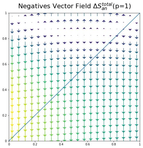
Hard negative examples are hard, but useful       9

                  +           Anchor        SCT Hard -       SHN Hard -

Fig. 3: Example triplets from the CAR and CUB datasets at the start of training.
The positive example is randomly selected from a batch, and we show the hard
negative example selected by SCT and SHN approach.

initialization from a pretrained model trained on ImageNet, which contains classes
such as birds and cars – images of birds all produce feature vectors that point in
generally the same direction in the embedding space, and likewise for images of cars.
    Figure 4 shows that the model trained with SCT approach has truly hard neg-
ative examples – ones that even as humans are difficult to distinguish. The negative
examples in the model trained with SHN approach, on the other hand, remain quite
random. This may be because when the network was initialized, these anchor-negative
pairs were accidentally very similar (very hard negatives) and were never included
in the semi-hard negative (SHN) optimization.

6    Experiments and Results

We run a set of experiments on the CUB200 (CUB) [24], CAR196 (CAR) [10], Stanford
Online Products (SOP) [18], In-shop Cloth (In-shop) [11] and Hotels-50K(Hotel) [20]
datasets. All tests are run on the PyTorch platform [14], using ResNet50 [7] architec-
tures, pre-trained on ILSVRC 2012-CLS data [15]. Training images are re-sized to 256
by 256 pixels. We adopt a standard data augmentation scheme (random horizontal flip
and random crops padded by 10 pixels on each side). For pre-processing, we normalize
the images using the channel means and standard deviations. All networks are trained
using stochastic gradient descent (SGD) with momentum 0. The batch size is 128
for CUB and CAR, 512 for SOP, In-shop and Hotel50k. In a batch of images, each
class contains 2 examples and all classes are randomly selected from the training data.
Empirically, we set λ=1 for CUB and CAR, λ=0.1 for SOP, In-shop and Hotel50k.
    We calculate Recall@K as the measurement for retrieval quality. On the CUB
and CAR datasets, both the query set and gallery set refer to the testing set. During
the query process, the top-K retrieved images exclude the query image itself. In the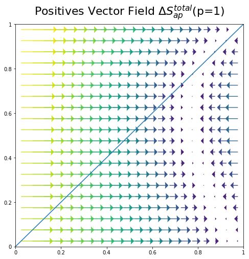
10      H. Xuan et al.

                  +            Anchor         SCT Hard -       SHN Hard -

Fig. 4: Example triplets from the CAR and CUB datasets at the end of training. The
positive example is randomly selected from a batch, and we show the hard negative
example selected by SCT and SHN approach.

Hotels-50K dataset, the training set is used as the gallery for all query images in the
test set, as per the protocol described by the authors in [20].

6.1   Hard negative triplets during training

Figure 5 helps to visualize what happens with hard negative triplets as the network
trains using the triplet diagram described in Section 3. We show the triplet diagram
over several iterations, for the HN approach (top), SHN approach (middle), and the
SCT approach introduced in this paper (bottom).
    In the HN approach (top row), most of the movements of hard negative triplets
coincide with the movement prediction of the vector field in the Figure 2 – all of the
triplets are pushed towards the bad minima at the location (1,1).
    During the training of SHN approach (middle row), it can avoid this local minima
problem, but the approach does not do a good job of separating the hard negative
pairs. The motion from the red starting point to the blue point after the gradient
update is small, and the points are not being pushed below the diagonal line (where
the positive example is closer than the negative example).
    SCT approach (bottom) does not have any of these problems, because the hard neg-
ative examples are more effectively separated early on in the optimization, and the blue
points after the gradient update are being pushed towards or below the diagonal line.
    In Figure 6, we display the percentage of hard triplets as defined in Section 3 in
a batch of each training iteration on CUB, CAR, SOP, In-shop Cloth and Hotels-
50k datasets (left), and compare the Recall@1 performance of HN, SHN and SCT
approaches (right). In the initial training phase, if a high ratio of hard triplets appear
in a batch such as CUB, CAR and Hotels-50K dataset, the HN approach converges
to the local minima seen in Figure 5.
Hard negative examples are hard, but useful 11 Fig. 5: Hard negative triplets of a batch in training iterations 0, 4, 8, 12. 1st row: Triplet loss with hard negative mining (HN); 2nd row: Triplet loss with semi hard negative mining (SHN). Although the hard negative triplets are not selected for training, their position may still change as the network weights are updated; 3rd row: Selectively Contrastive Triplet loss with hard negative mining (SCT). In each case we show where a set of triplets move before an after the iteration, with the starting triplet location shown in red and the ending location in blue. Fig. 6: Left: the percentage of hard triplets in a batch for SOP, In-shop Cloth and Hotels-50K datasets. Right: Recall@1 performance comparison between HN, SHN and SCT approaches.
12        H. Xuan et al.

                                    Hotel Instance                  Hotel Chain
           Method            R@1      R@10        R@100      R@1       R@3        R@5
     BATCH-ALL [20]256        8.1      17.6        34.8      42.5      56.4       62.8
     Easy Positive [27]256   16.3      30.5        49.9       -          -         -
           SHN256            15.1      27.2        44.9      44.9      57.5       63.0
           SCT256            21.5      34.9        51.8      50.3      61.0       65.9

Table 1: Retrieval performance on the Hotels-50K dataset. All methods are trained
with Resnet-50 and embedding size is 256.

    We find the improvement is related to the percentage of hard triplets when it
drops to a stable level. At this stage, there is few hard triplets in In-shop Cloth
dataset, and a small portion of hard triplets in CUB, CAR and SOP datasets, a
large portion of hard triplets in Hotels-50K dataset. In Figure 6, the model trained
with SCT approach improves R@1 accuracy relatively small improvement on CUB,
CAR, SOP and In-shop datasets but large improvement on Hotels-50K datasets with
respect to the model trained with the SHN approach in Table 1, we show the new
state-of-the-art result on Hotels-50K dataset, and tables of the other datasets are
shown in Appendix (this data is visualized in Figure 6 (right)).

6.2     Generalizability of SCT Features

Improving the recall accuracy on unseen classes indicates that the SCT features are
more generalizable – the features learned from the training data transfer well to the
new unseen classes, rather than overfitting on the training data. The intuition for
why the SCT approach would allow us to learn more generalizable features is because
     forcing the network to give the same feature representation to very different
examples from the same class is essentially memorizing that class, and that is not
likely to translate to new classes. Because SCT uses a contrastive approach on hard
negative triplets, and only works to decrease the anchor-negative similarity, there is
less work to push dis-similar anchor-positive pairs together. This effectively results
in training data being more spread out in embedding space which previous works
have suggested leads to generalizable features [25,27].
     We observe this spread out embedding property in the triplet diagrams seen in
Figure 7. On training data, a network trained with SCT approach has anchor-positive
pairs that are more spread out than a network trained with SHN approach (this
is visible in the greater variability of where points are along the x-axis), because
the SCT approach sometimes removes the gradient that pulls anchor-positive pairs
together. However, the triplet diagrams on test set show that in new classes the
triplets have similar distributions, with SCT creating features that are overall slightly
higher anchor-positive similarity.
     A different qualitative visualization in Figure 8, shows the embedding similarity
visualization from [19], which highlights the regions of one image that make it look sim-
ilar to another image. In the top set of figures from the SHN approach, the blue regions
Hard negative examples are hard, but useful 13
Fig. 7: We train a network on the CAR dataset with the SHN and SCT approach
for 80 epochs. Testing data comes from object classes not seen in training. We make
a triplet for every image in the training and testing data set, based on its easiest
positive (most similar same class image) and hardest negative (most similar different
class image), and plot these on the triplet diagram. We see the SHN (left) have a
more similar anchor-positive than SCT (right) on the training data, but the SCT
distribution of anchor-positive similarities is greater on images from unseen testing
classes, indicating improved generalization performance.
that indicate similarity are diffuse, spreading over the entire car, while in the bottom
visualization from the SCT approach, the blue regions are focused on specific features
(like the headlights). These specific features are more likely to generalize to new, unseen
data, while the features that represent the entire car are less likely to generalize well.
7 Discussion
Substantial literature has highlighted that hard negative triplets are the most informa-
tive for deep metric learning – they are the examples where the distance metric fails to
accurately capture semantic similarity. But most approaches have avoided directly op-
timizing these hard negative triplets, and reported challenges in optimizing with them.
This paper introduces the triplet diagram as a way to characterize the effect
of different triplet selection strategies. We use the triplet diagram to explore the
behavior of the gradient descent optimization, and how it changes the anchor-positive
and anchor-negative similarities within triplet. We find that hard negative triplets
have gradients that (incorrectly) force negative examples closer to the anchor, and
situations that encourage triplets of images that are all similar to become even more
similar. This explains previously observed bad behavior when trying to optimize with
hard negative triplets.
We suggest a simple modification to the desired gradients, and derive a loss
function that yields those gradients. Experimentally we show that this improves the14 H. Xuan et al.
(a) SHN (b) SHN
(c) SCT (d) SCT
Fig. 8: The above figures show two query images from the CAR dataset (middle left
in each set of images) , and the top five results returned by our model trained with
hard negative examples. The Similarity Visualization approach from [19] show what
makes the query image similar to these result images (blue regions contribute more to
similarity than red regions). In all figures, the visualization of what makes the query
image look like the result image is on top, and the visualization of what makes the
result image look like the query image is on the bottom. The top two visualizations (a)
and (b) show the visualization obtained from the network trained with SHN approach,
while the bottom two visualizations (c) and (d) show the visualization obtained
from the network trained with SCT approach. The heatmaps in the SCT approach
visualizations are significantly more concentrated on individual features, as opposed
to being more diffuse over the entire car. This suggests the SCT approach learns
specific semantic features rather than overfitting and memorizing entire vehicles.
convergence for triplets with hard negative mining strategy. With this modification,
we no longer observe challenges in optimization leading to bad local minima and show
that hard-negative mining gives results that exceed or are competitive with state of
the art approaches. We additionally provide visualizations that explore the improved
generalization of features learned by a network trained with hard negative triplets.
Acknowledgements: This research was partially funded by the Department of Energy,
ARPA-E award #de-ar0000594, and NIJ award 2018-75-CX-0038. Work was partially
completed while the first author was an intern with Microsoft Bing Multimedia team.Hard negative examples are hard, but useful 15
References
1. Cakir, F., He, K., Xia, X., Kulis, B., Sclaroff, S.: Deep metric learning to rank. In: The
IEEE Conference on Computer Vision and Pattern Recognition (CVPR) (June 2019)
2. Faghri, F., Fleet, D.J., Kiros, J.R., Fidler, S.: Vse++: Improving visual-semantic
embeddings with hard negatives. In: Proceedings of the British Machine Vision
Conference (BMVC) (2018)
3. Ge, J., Gao, G., Liu, Z.: Visual-textual association with hardest and semi-hard negative
pairs mining for person search. arXiv preprint arXiv:1912.03083 (2019)
4. Ge, W.: Deep metric learning with hierarchical triplet loss. In: Proc. European
Conference on Computer Vision (ECCV) (September 2018)
5. Goldberger, J., Hinton, G.E., Roweis, S.T., Salakhutdinov, R.R.: Neighbourhood
components analysis. In: Saul, L.K., Weiss, Y., Bottou, L. (eds.) Advances in Neural
Information Processing Systems 17, pp. 513–520. MIT Press (2005)
6. Harwood, B., Kumar, B., Carneiro, G., Reid, I., Drummond, T., et al.: Smart mining
for deep metric learning. In: Proceedings of the IEEE International Conference on
Computer Vision. pp. 2821–2829 (2017)
7. He, K., Zhang, X., Ren, S., Sun, J.: Deep residual learning for image recognition. In: Proc.
IEEE Conference on Computer Vision and Pattern Recognition (CVPR) (June 2016)
8. Hermans*, A., Beyer*, L., Leibe, B.: In Defense of the Triplet Loss for Person
Re-Identification. arXiv preprint arXiv:1703.07737 (2017)
9. Kim, W., Goyal, B., Chawla, K., Lee, J., Kwon, K.: Attention-based ensemble for
deep metric learning. In: Proc. European Conference on Computer Vision (ECCV)
(September 2018)
10. Krause, J., Stark, M., Deng, J., Fei-Fei, L.: 3d object representations for fine-grained
categorization. In: 4th International IEEE Workshop on 3D Representation and
Recognition (3dRR-13). Sydney, Australia (2013)
11. Liu, Z., Luo, P., Qiu, S., Wang, X., Tang, X.: Deepfashion: Powering robust clothes
recognition and retrieval with rich annotations. In: Proceedings of IEEE Conference
on Computer Vision and Pattern Recognition (CVPR) (June 2016)
12. Movshovitz-Attias, Y., Toshev, A., Leung, T.K., Ioffe, S., Singh, S.: No fuss distance
metric learning using proxies. In: Proc. International Conference on Computer Vision
(ICCV) (Oct 2017)
13. Opitz, M., Waltner, G., Possegger, H., Bischof, H.: Bier - boosting independent embed-
dings robustly. In: Proc. International Conference on Computer Vision (ICCV) (Oct 2017)
14. Paszke, A., Gross, S., Chintala, S., Chanan, G., Yang, E., DeVito, Z., Lin, Z., Desmaison,
A., Antiga, L., Lerer, A.: Automatic differentiation in pytorch. In: NIPS-W (2017)
15. Russakovsky, O., Deng, J., Su, H., Krause, J., Satheesh, S., Ma, S., Huang, Z., Karpathy,
A., Khosla, A., Bernstein, M., Berg, A.C., Fei-Fei, L.: ImageNet Large Scale Visual
Recognition Challenge. International Journal of Computer Vision (IJCV) 115(3),
211–252 (2015)
16. Schroff, F., Kalenichenko, D., Philbin, J.: Facenet: A unified embedding for face
recognition and clustering. In: Proc. IEEE Conference on Computer Vision and Pattern
Recognition (CVPR) (June 2015)
17. Sohn, K.: Improved deep metric learning with multi-class n-pair loss objective. In:
Advances in Neural Information Processing Systems. pp. 1857–1865 (2016)
18. Song, H.O., Xiang, Y., Jegelka, S., Savarese, S.: Deep metric learning via lifted
structured feature embedding. In: Proc. IEEE Conference on Computer Vision and
Pattern Recognition (CVPR) (2016)16 H. Xuan et al.
19. Stylianou, A., Souvenir, R., Pless, R.: Visualizing deep similarity networks. In: IEEE
Winter Conference on Applications of Computer Vision (WACV) (January 2019)
20. Stylianou, A., Xuan, H., Shende, M., Brandt, J., Souvenir, R., Pless, R.: Hotels-50k: A
global hotel recognition dataset. In: AAAI Conference on Artificial Intelligence (2019)
21. Suh, Y., Han, B., Kim, W., Lee, K.M.: Stochastic class-based hard example mining
for deep metric learning. In: The IEEE Conference on Computer Vision and Pattern
Recognition (CVPR) (June 2019)
22. Wang, C., Zhang, X., Lan, X.: How to train triplet networks with 100k identities? In:
Proceedings of the IEEE International Conference on Computer Vision Workshops.
pp. 1907–1915 (2017)
23. Wang, X., Han, X., Huang, W., Dong, D., Scott, M.R.: Multi-similarity loss with
general pair weighting for deep metric learning. In: Proceedings of the IEEE Conference
on Computer Vision and Pattern Recognition. pp. 5022–5030 (2019)
24. Welinder, P., Branson, S., Mita, T., Wah, C., Schroff, F., Belongie, S., Perona, P.: Caltech-
UCSD Birds 200. Tech. Rep. CNS-TR-2010-001, California Institute of Technology (2010)
25. Wu, Z., Xiong, Y., Yu, S.X., Lin, D.: Unsupervised feature learning via non-parametric
instance discrimination. In: The IEEE Conference on Computer Vision and Pattern
Recognition (CVPR) (June 2018)
26. Xuan, H., Souvenir, R., Pless, R.: Deep randomized ensembles for metric learning. In:
Proc. European Conference on Computer Vision (ECCV) (September 2018)
27. Xuan, H., Stylianou, A., Pless, R.: Improved embeddings with easy positive triplet
mining. In: The IEEE Winter Conference on Applications of Computer Vision (WACV)
(March 2020)
28. Yu, B., Liu, T., Gong, M., Ding, C., Tao, D.: Correcting the triplet selection bias for
triplet loss. In: Proceedings of the European Conference on Computer Vision (ECCV).
pp. 71–87 (2018)
29. Zhang, X., Yu, F.X., Kumar, S., Chang, S.F.: Learning spread-out local feature descrip-
tors. In: The IEEE International Conference on Computer Vision (ICCV) (Oct 2017)Hard negative examples are hard, but useful 17
Appendix
.1 Similarity after gradient updating(NCA-based triplet loss)
new new
The following derivations show how to get Sap and San in equation 7 and 8 with
new new new
updated and unnormalized fa ,fp ,fn in equation 4, 5 and 6.
|
new
Sap =fanew fpnew
=(1+β 2)fa|fp +βfa|fa +βfp|fp −βfn|fp −β 2fn|fa (14)
2 2
=(1+β )Sap +2β−βSpn −β San
|
new
San =fanew fnnew
=(1+β 2)fa|fn −βfa|fa −βfn|fn +βfp|fn −β 2fp|fa (15)
2 2
=(1+β )Sap −2β+βSpn −β Sap
new
For the calculation of Sap , we construct two hyper-planes: Pap spanned by fa
and fp, and Pan spanned by fa and fn. On Pap, fp can be decomposed into two
ak
components: fp (the direction along fa) and fpa⊥(the direction vertical to fa). On Pan,
ak
fn can be decomposed into two components: fn (the direction along fa) and fna⊥(the
direction vertical to fa). Then the Spn should be:
Spn =fp|fn
=(fpak +fpa⊥)(fnak +fna⊥) (16)
q p
=SapSan +γ 1−Sap 2 2
1−San
f a⊥ f a⊥
p n
where γ = kf a⊥ a⊥ , which represents the projection factor between Pap and Pan .
p kkfn k
When fa, fn, and fp are close enough so that locally the hypersphere is a plane, then
γ is the dot-product of normalized vector from fa to fp and fa to fn. If fp,fa,fn are
co-planer then γ =1, and if moving from fa to fp is orthogonal to the direction from
fa to fn, then γ =0.
.2 Norm of updated features(NCA-based triplet loss)
The following derivation shows how to derive kfanew k, kfpnew k and kfnnew k in equa-
tion 9 and 10. On Pap, gp can be decomposed into the direction along fp and the
direction vertical to fp. On Pan, gn can be decomposed into the direction along fn
and the direction vertical to fn. Then,
kfpnew k2 =(1+βSap)2 +β 2(1−Sap
2
) (17)
new 2 2 2 2
kfn k =(1−βSan) +β (1−San ) (18)18 H. Xuan et al.
Dataset CUB CAR
Method R@1 R@2 R@4 R@8 R@1 R@2 R@4 R@8
Triplet-Semihard64 42.6 55.03 66.4 77.2 51.5 63.8 73.5 82.4
Lifted64 43.6 56.6 68.6 79.6 53.0 65.7 76.0 84.3
Clustering64 49.8 61.4 71.8 81.9 58.1 70.6 80.3 87.8
SmartMining64 49.8 62.3 74.1 83.3 64.7 76.2 84.2 90.2
ProxyNCA64 49.2 61.9 67.9 72.4 73.2 82.4 86.4 88.7
N-pair64 51.9 64.3 74.9 83.2 71.1 79.7 86.5 91.6
SHN64 56.2 67.0 78.0 86.1 68.2 77.8 85.5 91.0
SCT64 57.6 69.8 79.3 87.2 73.2 82.4 88.4 93.0
Table 2: Retrieval Performance on the CUB and CAR datasets comparing to the
best reported results with embedding dimension 64 trained on ResNet50.
Dataset SOP In-shop
Method R@1 R@10 R@100 R@1 R@10 R@20
BIER [13]512 72.7 86.5 94.0 76.9 92.8 95.2
ABE [9]512 76.3 88.4 94.8 87.3 96.7 97.9
FastAP [1]512 76.4 89.0 95.1 90.9 97.7 98.5
MS [23]512 78.2 90.5 96.0 89.7 97.9 98.5
EasyPositive [27]512 78.3 90.7 96.3 87.8 95.7 96.8
SHN512 80.8 92.0 96.9 90.1 97.3 98.2
SCT512 81.6 92.3 96.7 90.0 97.3 98.1
Table 3: Retrieval Performance on the SOP and In-shop datasets comparing to the
best reported results with embedding dimension 512 trained on ResNet50
On Pap, ga can be decomposed into 3 components: component in the plane and along
fa, component in the plane and vertical fa, and component vertical to Pap. Then,
kfanew k2 =(1+βSap −βSan)2
q p
+(β 1−Sap2 −γβ 1−S 2 )2 (19)
an
p p
2 2 2
+(β 1−γ 1−San)
.3 Gradient updates(margin-based triplet loss)
The main paper uses NCA-based triplet loss. Another margin-based triplet-loss
function is derived to guarantee a specific margin. This can be expressed in terms
of fa,fp,fn as:
L=max(kfa −fpk2 −kfa −fnk2 +α,0)=max(D,0) (20)Hard negative examples are hard, but useful 19
(
−β(fa −fp)
∂L if D >0
gp = = ∂fp (21)
0 otherwise
(
∂L β(fa −fn) if D >0
gn = ∂f = (22)
n
0 otherwise
(
∂L β(fn −fp) if D >0
ga = ∂f = (23)
a
0 otherwise
where D = (kfa − fpk2 − kfa − fnk2 + α) and β = 2. For simplicity, in the following
discussion, we set D > 0 for margin-based triplet loss. Then we can get the fanew ,
fpnew and fnnew and their norm:
fpnew = fp +β(fa −fp) =(1−β)fp +βfa (24)
new
fn = fn −β(fa −fn) =(1+β)fn −βfa (25)
new
fa = fa −βfn +βfp (26)
kfpnew k2 =(1−β+βSap)2 +β 2(1−Sap
2
) (27)
new 2 2 2 2
kfn k =(1+β−βSan) +β (1−San ) (28)
kfanew k2 =(1+βSap −βSan)2
q p
+(β 1−Sap2 −γβ 1−S 2 )2 (29)
an
p p
2 2 2
+(β 1−γ 1−San)
new new
The updated similarity Sap and San will be:
new
Sap =(1−β+β 2)Sap +2β−β 2 −β(1−β)Spn −β 2San (30)
new
San =(1+β+β 2)San −2β−β 2 +β(1+β)Spn −β 2Sap (31)
new new
Comparing to the Sap and San in equation 7 and 8 of main paper, margin-based
triplet loss behavior is similar to the NCA-based triplet loss. And we simulate the
∆Sap and ∆San with the margin-based triplet loss in figure 9. These plots show that
the behavior of problematic regions are qualitatively similar for both methods with
different values of entanglement strength p.
.4 More Results on other dataset
We also compare our results with state-of-the-art embedding approaches such as
BIER [13],ABE [9],FaseAP [1] Multi-Similarity [23] and Easy Positive [27] on SOP [18]
and In-shop [11] dataset. Tables 3 shows the SC-triplet loss outperforms the best
previously reported results on the SOP dataset.20 H. Xuan et al.
Lnca Lmargin
total total
Fig. 9: Numerical simulation for ∆Sap, ∆San, ∆Sap and ∆San change of Lnca
margin
and L with p=0.5,1.0.You can also read