IMPACT OF VARIABLE SPEED ON COLLECTIVE MOVEMENT OF ANIMAL GROUPS
←
→
Page content transcription
If your browser does not render page correctly, please read the page content below
I MPACT OF VARIABLE S PEED ON C OLLECTIVE M OVEMENT OF
                                                                       A NIMAL G ROUPS

                                                      Pascal P. Klamser1,2 , Luis Gómez-Nava1,3 , Tim Landgraf3,4 , Jolle W. Jolles5 , David Bierbach3,6,7 , and Pawel
arXiv:2106.00959v2 [physics.bio-ph] 17 Jun 2021

                                                                                                     Romanczuk1,2,3

                                                      1
                                                        Institute for Theoretical Biology, Department of Biology, Humboldt Universität zu Berlin, Berlin, Germany.
                                                                         2
                                                                           Bernstein Center for Computational Neuroscience, 10115 Berlin, Germany.
                                                              3
                                                                Cluster of Excellence, Science of Intelligence, Technische Universität Berlin, Berlin, Germany.
                                                              4
                                                                Department of Mathematics and Computer Science, Freie Universität Berlin, Berlin, Germany.
                                                  5
                                                    Center for Ecological Research and Forestry Applications (CREAF), Campus de Bellaterra (UAB), Barcelona, Spain.
                                                  6
                                                    Department of Biology and Ecology of Fishes, Leibniz-Institute of Freshwater Ecology and Inland Fisheries, Berlin,
                                                                                                            Germany.
                                                     7
                                                       Faculty of Life Sciences, Albrecht Daniel Thaer-Institute of Agricultural and Horticultural Sciences, Humboldt
                                                                                            Universität zu Berlin, Berlin, Germany.

                                                                                                        June 18, 2021

                                                                                                        A BSTRACT

                                                          The collective dynamics and structure of animal groups has attracted the attention of scientists from
                                                          different disciplines. A variety of agent-based models has been proposed to account for the emergence
                                                          of coordinated collective behavior from simple interaction rules. A common, simplifying assumption
                                                          of such collective movement models, is the consideration of individual agents moving with a constant
                                                          speed. In this work we critically re-asses this assumption underlying a vast majority of collective
                                                          movement models. First, we discuss experimental data showcasing the omnipresent speed variability
                                                          observed in different species of live fish and artificial agents (RoboFish). Based on theoretical
                                                          considerations accounting for inertia and rotational friction, we derive a functional dependence of the
                                                          turning response of individuals on their instantaneous speed, which is confirmed by experimental data.
                                                          We investigate how the interplay of variable speed and speed-dependent turning affects self-organized
                                                          collective behavior by implementing an agent-based model which accounts for both effects. We
                                                          show, that besides average speed, the individual speed variability may have a dramatic impact on
                                                          the emergent collective dynamics, as two groups differing only in their speed variability, and being
                                                          otherwise identical in all other behavioral parameters, can be in two fundamentally different stationary
                                                          states (polarized versus disordered). We find that the local coupling between group polarization
                                                          and individual speed is strongest at the order-disorder transition, and that, in contrast to fixed speed
                                                          models, the group’s spatial extent does not have a maximum at the transition. Furthermore, we
                                                          demonstrate a decrease in polarization with group size for groups of individuals with variable speed,
                                                          and a sudden decrease in mean individual speed at a critical group size (N=4 for Voronoi interactions)
                                                          linked to a topological transition from an all-to-all to a distributed spatial interaction network. Overall,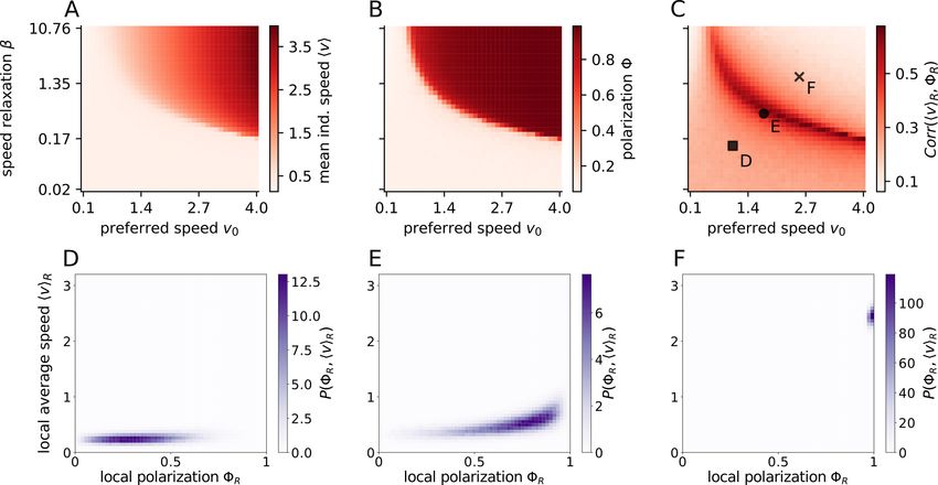
J UNE 18, 2021

         our work highlights the importance to account for fundamental kinematic constraints in general, and
         variable speed in particular, when modeling self-organized collective dynamics.

1   Introduction

The emergent, highly coordinated, collective movements as observed in schools of fish, flocks of birds, or insect swarms,
are fascinating examples of biological self-organization. Although our understanding of these collective systems has
been significantly advanced over the past years through diverse research efforts in biology [1, 2, 3, 4, 5], mathematics
[6, 7, 8], computer science [9, 10], engineering [11, 12], and statistical physics [13, 14, 15, 16, 17], many fundamental
questions remain open, for example regarding the underlying interaction networks (”Who interacts with whom?”)
[18, 19, 20].
In addition to the analysis of empirical observations [14, 19], mathematical models are an important tool for studying
self-organization and collective behavior, and have been instrumental in uncovering general principles of how robust,
large-scale coordination can emerge from simple, local interactions between self-propelled agents [21, 10, 22].
When formulating models, in general and for animal collectives, one has to balance between simplicity/generality and
detailed resemblance to experimental systems. From a statistical physics point of view, it is viable to assume some sort
of universality of the collective dynamics even in far-from-equilibrium situations. Thus, as long as the model accounts
for crucial aspects of the microscopic dynamics, other microscopic details become irrelevant for the macroscopic
behavior for sufficiently large systems over a long temporal scale. However, 1) there is no general way to tell when the
system is sufficiently large, and 2) animal groups consist of tens to hundreds, rarely thousands or more, individuals.
Therefore, animal collectives should be rather viewed as mesoscopic systems, where the actual details of individual
movement behavior may play an important role [23], and caution is advised when simplifying modeling assumptions.
A particularly prominent simplification often encountered in flocking models is the assumption of constant speed of
individual agents, used in a vast majority of flocking models [24, 13, 25, 26]; for exceptions see e.g. [27, 28, 29, 30, 31].
However, in general animals are able to flexibly modify their movement speed. Thus, speed adaptation due to
environmental factors or social interactions [2] – ignored in constant speed models – may play a decisive role in shaping
the ability of groups to coordinate their movement and in the resulting structure of moving animal groups [32]. In fact,
experiments demonstrated that speed influences the collective behavior strongly, via a coupling to polarization/alignment
[28, 27, 25, 3, 33, 32] which could also be shown on the local scale [28], i.e. regions in the shoal with faster fish are
more polarized. While in former simulation studies the speed influenced the turning rate or modified the assumed
social forces, mostly fixed speed models were used rendering the speed to a mere parameter and not a changing
variable [24, 25, 34, 3]. It has been shown that a variable speed of individuals may lead to qualitatively new, emergent
phenomena on the group level as for example bi-stable behavior with respect to polarization, i.e. a co-existence of stable
ordered states and disordered collective states at high densities [27, 28]. These findings demonstrate the important role
of feedbacks between speed, turning, and social interactions for the emergence and stability of collective states. Here,
in the context of the collective movement of self-propelled agents that are meant to represent animal groups in the real
world, we will discuss how inertia and friction link those properties.
In general, individuals in a group can differ in persistent behavioral traits (animal personality) which may induce
between-individual variance in speed [35, 3, 36, 37]). The inter-individual variability in preferred movement speed
has been found to influence cohesion and polarization of groups [3, 33], and it has been shown to decrease in larger
groups [37]. However, already in behaviorally homogeneous groups, with individuals having similar preferred speeds,
the instantaneous speed of single individuals will dynamically vary over time due to its direct response to social
and/or environmental cues, as well as due to internal decision processes (”internal” fluctuations). Both types of speed
variability will be important for the collective movement dynamics [27]. We focus on the investigation of the role
of within-individual speed variability on emergent, self-organized collective movement using an agent-based model.
In particular, we demonstrate how accounting for the ability of individuals to dynamically modulate their speed has

                                                             2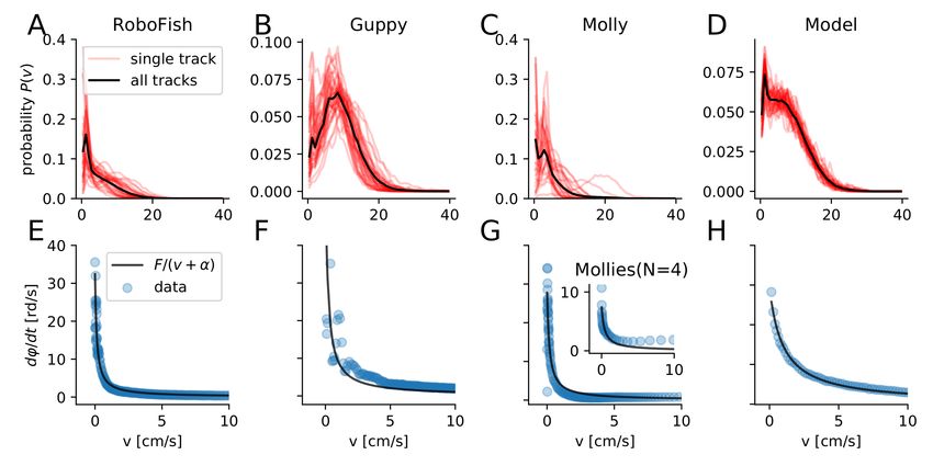
J UNE 18, 2021

profound effects on the group behavior, which are highly relevant for experimental observations of collective animal
movement.
In the following, we will first provide an experimental motivation for our modeling ansatz by analyzing speed variability
in schooling fish and providing evidence for coupling between turning behavior and instantaneous speed, which can
be theoretically understood by considering self-propelled movement with inertia. Inspired by these results we will
then investigate an agent-based model of collective movement with variable speed and demonstrate how the ability of
individuals to flexibly adapt their speed in response to social interactions and fluctuations has major consequence for
the emergent collective dynamics.

2     Methods

2.1   Experimental Data

In order to show within-individual variability in movement speeds, we analyzed previously published data sets of
individual movement for two different fish species Poecilia reticulata (Trinidadian guppy, [33]) , Poecilia formosa
(clonal Amazon molly, [36])) as well as a biomimetic robot (’RoboFish’, [3]). For the Amazon molly, we further
included a data set in which groups of 4 fish were observed [38]. All data sets consist of positional tracking data from
laboratory observations with a sampling frame rate of 30 fps, circular or rectangular arenas smaller than 1 square meter
in size and only female fish, as summarized in Tab. 1 and in more detail explained in SI Sec. I.

                               RoboFish              Guppy            Molly (single ind.)   Mollies (groups of 4)
      Species                        –            Poecilia reticulata                Poecilia formosa
      # of tracks                   39                      40                   35                      32
      Observation time           10 min                  10 min                6 min                   5 min
      Arena dimensions         88×88 cm                88×88 cm          48.5cm diameter            60×30 cm
      Water depth                 7.5 cm                 7.5 cm                3 cm                    5 cm
      Frame acquisition          30 FPS                  30 FPS              30 FPS                  30 FPS
      Sex                            –                   female               female                  female
      Tracking method       BioTracker [39]            BioTracker        Ethovision (10.1)      Ethovision (XT12)
      Reference                          Jolles et al. [33]             Bierbach et al. [36]     Doran et al. [38]
Table 1: List of previously published tracking data used in our analysis. The table lists major characteristics of the
datasets we used to show within-individual speed variability. The # of tracks indicates the number of individual tracks
used for the analysis. Du to the initial study designs and questions, tracks may represent repeated measures of the same
(Guppy: 20 individuals, RoboFish 1 replica) or different individuals (Molly single ind, Molly groups: 8 with 4 ind. per
group). Please find exact study designs in the respective references.

2.2   Processing of trajectories
                                                                                                                      T
The tracking data obtained for the different species and the robotic fish encodes the position xi (t) = xi (t), yi (t)
of the individual i for each frame t. We approximate the velocity of each individual from subsequent positions by
computing:
                                                          xi (t + ∆t) − xi (t)
                                        vi,x (t + ∆t) =                        , .                                   (1)
                                                                  ∆t

We can approximate the direction of motion of individual i by ϕi (t) = arctan2 vi,y (t), vi,x (t) . In a similar way as
in Eq. (1) we compute the angular speed ϕ̇(t) of each individual.

                                                            3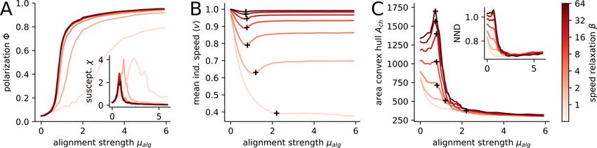
J UNE 18, 2021

2.3   Fundamental relations between speed and turning

The fundamental equation of motion for a self-propelled agent i reads:
                                                    dvi (t)  1
                                                            = Fi (t)                                                     (2)
                                                      dt     m
with vi as the velocity vector of the agent, m it’s mass and Fi being total force acting on it. Please note that, in the
following, we omit the explicit time dependence for simplicity. The velocity vector can be expressed via the speed vi
and the heading angle ϕi to vi = vi [cos ϕi , sin ϕi ]T = vi êv,i . We can reformulate (in detail shown in SI Sec. II) the
velocity dynamics in terms of speed and heading angle dynamics [40] to
                                       dvi   Fi
                                           =    · êv,i                                                                  (3)
                                        dt   m                          "        #
                                       dϕi    Fi                          cos ϕi
                                           =       · êϕ,i with êv,i =            .                                     (4)
                                        dt   vi m                         sin ϕi

Therefore, without any further assumptions, we see that the turning is inversely proportional to the current speed, i.e.
dϕi /dt ∝ 1/vi . However, the inverse proportionality results in instantaneous turning for vi = 0, which is unrealistic
and is caused by assuming a point-like object. To provide a simple correction for this unreasonable assumption, we
follow [41] and introduce a rotational friction force acting on the velocity

                                             dvi     1            dϕi
                                                  =       Fi − α       êϕ,i                                        (5)
                                              dt     m             dt
with α as rotational friction coefficient. If we repeat the steps from above analogously, the speed dynamics remain
unchanged (Eq. 3) but the change in heading angle reads now:
                                                dϕi       Fi
                                                    =            · êϕ,i .                                               (6)
                                                 dt   (vi + α) m

In the context of self-propelled agents, the above relation implies that the turning rate of an individual, in response to a
force Fi acting on the agent or generated by the agent itself, depends on its speed vi . For a constant force |Fi | = const.,
faster agents will turn slower. Alternatively, in order to turn at the same rate, individuals moving at different speeds
have to adjust the strength of their turning force linearly with their current speed. We emphasize that this fundamental
relation, ignored in most models of collective behavior explicitly modeling turning rates, holds both for fixed speeds
vi := v0,i = const., as well as for variable speeds vi := vi (t).

2.4   Fitting experimental data

We used the least square fitting method to obtain the best fitting functional dependency between v = |v| and ϕ̇. We
considered the two equations (4) and (6), introduced in the preceding Sec. 2.3, and thus minimizing the squared
difference of the data to dϕ/dt = Fϕ /v and dϕ/dt = Fϕ /(v + α) respectively. Here we treat the force in angular
direction Fϕ = F · êϕ , and the rotational friction coefficient α as parameters. Since Eq. 6 has one parameter more (α),
we compared both fits using the Akaike Information Criterion (AIC) [42] and the Bayesian Information Criterion (BIC)
[43]. Those criteria penalize a larger number of parameters and therefore prevent overfitting.

2.5   The Model

As explained in section 2.3, the model we use mimics the movement behavior of real fish by obeying fundamental
physics relations (inertia and friction). This is mathematically expressed in Eqs. 5, 6. Additionally, the interaction
between fish is motivated by the continuous version of a well established three zone model (already introduced with
fixed speed in [22]). Thus, the force acting on an individual i has a self-propulsion term (including noise) and a social

                                                             4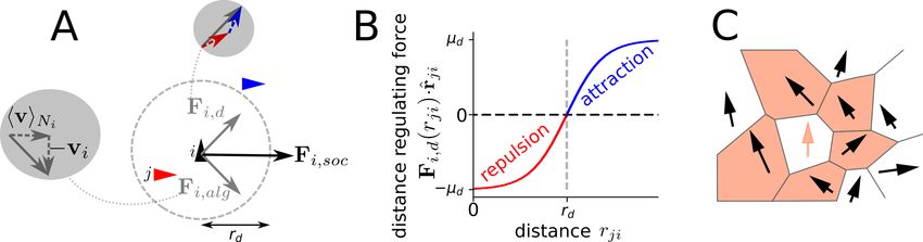
J UNE 18, 2021

Figure 1: Implementation of social interactions. A focal agent (black triangle) responds to neighbors (red and blue
triangle) via a velocity alignment force Fi,alg , which aims at minimizing the velocity difference to the mean neighbor
velocity hviNi , and a distance regulating force Fi,d , their sum corresponds to the social force Fi,soc (A). For simplicity
the distance regulating force has a sigmoidal distance dependence: it is repulsive for distances closer, and attractive for
distances larger than a preferred distance rd (A, B). The neighborhood of a focal agent (red arrow) is defined by its
Voronoi neighbors (black arrows in red cells, C).

term. We can express this as: Fi (t) = Fi,sp (t) + Fi,social (t). The self-propulsion force takes into account two main
factors: 1) the tendency of an individual to keep a preferred speed v0 and 2) the fluctuations on the linear speed v and
the angular speed ϕ̇

                                                  p                           p
                       Fi,sp (t) = β v0 − vi (t) + 2Dv ξv (t) êv,i +            2Dϕ ξϕ (t) êϕ,i ,                   (7)

where β is the speed relaxation coefficient, leading to the relaxation of the speed towards the preferred speed v0 in
the absence of other perturbations with the time constant τv = β −1 . Dv and Dϕ are diffusion coefficients setting the
noise intensity in v and ϕ, respectively, whereas ξv and ξϕ are independent, Gaussian white noise processes. The social
interactions are explained in detail in the following.

2.5.1   Social interactions

We consider a social force that combines two fundamental types of interactions among individuals: 1) an alignment
force Fi,alg and 2) a distance-regulating force Fi,d (Fig. 1A, B). Thus, we can express the total social force as
Fi,social (t) = Fi,alg (t) + Fi,d (t). We use Voronoi tesselation to define the neighborhood of a focal individual i, which
is labeled as Ni (Fig. 1C). A Voronoi interaction network can, on the one hand, be efficiently computed, while on the
other hand it also shows a good approximation with visual interaction networks [44]. The mathematical expression of
the alignment force is:
                                                            1 X
                                            Fi,alg (t) =         µalg vji (t),                                            (8)
                                                           |Ni |
                                                               j∈Ni

where µalg is the alignment strength and vji (t) = vj (t) − vi (t). The distance-regulating social force assumes a
preferred distance rd that individuals try to maintain between each other. It is defined as:

                                             1 X
                               Fi,d (t) =           µd tanh md rji (t) − rd r̂ji (t),                          (9)
                                           |Ni |
                                                j∈Ni

where r̂ji = (rj − ri )/|rj − ri | is a unitary vector from agent i to agent j, rji = |rj − ri |, µd is the strength of the
force and md is the slope of the change from repulsion (rji < rd ) and attraction (rji > rd ) (Fig. 1B). In principle, it is
possible to extract a specific functional form of the repulsion and attraction interaction from experimental data [2, 45, 30].
However, these functions will likely depend on the species and the ecological context, whereas the qualitative role of
variable speed discussed below does not depend on the specific choice of the functional form of the inter-individual

                                                              5
J UNE 18, 2021
Figure 2: Speed and turning of individuals. The speed probability distributions P (v) for the experimental data
(RoboFish, guppy, molly) and for model simulations of individuals (A-D). Red transparent lines represent single tracks
and the solid black line is the distribution of all tracks summarized. The absolute turning rate ϕ̇ as a function of
the speed v for the different individuals(E-H). For mollies we also show the relation between turning rate speed of
individuals swimming in groups of N = 4 (inset G). The parameters of the model simulations (described in Section 2.5)
are listed in Tab. S4 and those of the model fits in Tab. S3.
attraction-repulsion interactions. Therefore, for the sake of simplicity and generality, we have chosen a rather simple
(sigmoidal) distance dependence for the distance regulating force controlled by only three parameters (µ, md , rd ), with
the key property being a finite preferred distance rd , which individuals try to keep to their neighbors.
2.5.2 The equations of motion
By considering the self-propulsion and social forces described above, we can write the explicit equations of motion for
individuals, which resemble the equations in [27]:
dvi (t) p
= β v0 − vi (t) + Fi,v (t) + 2Dv ξv (t) (10)
dt
dϕi (t) 1 p
= Fi,ϕ (t) + 2Dϕ ξϕ (t) , (11)
dt vi (t) + α
with Fi,v (t) = Fi,social (t) · êv,i (t) being the projection of the social force on the heading direction êv,i and Fi,ϕ (t) =
Fi,social (t) · êϕ,i (t) being the projection of the social force on the turning direction êϕ,i .
3 Results
3.1 Experimental Data of Individual Fish
The speed variability and the dependence of turning on the instantaneous speed are fundamental characteristics of the
movement of individual self-propelled agents (c.f. [46, 41]). In Fig. 2A-C,E-G, we show the corresponding experimental
results obtained from analyzing the trajectories of two different fish species (guppies & mollies) and the robotic fish.
We show that live as well as artificial agents exhibit the same qualitative behavior: 1) non-negligible speed variability
6J UNE 18, 2021
RoboFish Guppy Molly Mollies(N=4) Model
aic bic aic bic aic bic aic bic aic bic
dϕ
dt= F/v 71 72 1170 1173 595 598 73 75 229 231
dϕ
dt= F/(v + α) -24 -22 523 530 316 322 11 15 -107 -102
Table 2: Statistical model comparison. Akaike (aic) and Baysian (bic) information criterion for a model without
( dϕ dϕ
dt = F/v) and with ( dt = F/(v + α)) turning-friction α for each model-species. The values of the parameters α
and F are listed in Tab. S3.
and 2) decrease of turning rate with increasing speed. The latter, in particular, can be linked to fundamental kinematic
constraints of inertial motion discussed above. We apply the same analysis on trajectories of our model simulation,
which produces the same characteristics Fig. 2D,H.
We find for all cases a speed distribution that shows a strong variation in speed (Fig. 2A-D). The Coefficient of variation
(COV(v) = σv /hvi) of the speed is about 1, i.e. the speed variation is as large as the mean speed. The results of the
single track analysis are: COV(v) = 0.92 ± 28 (RoboFish), 0.57 ± 0.1 (guppy), 0.92 ± 0.78 (single molly), 0.68 ± 0.03
(model).
Thus, speed variation typically neglected by fixed speed models, is clearly evident in the experimental data and
accounted for in our variable speed model, Fig. 2D. Accounting for variable speed is important, as due to inertia the
turning ability of any object is inversely proportional to its speed dϕ/dt = F/v. If we take turning friction into account
(friction coefficient α, see Methods), the turning rate becomes dϕ/dt = F/(v + α). The inverse speed dependence of
the turning rate is observable for all 4 cases (Fig. 2E-H). A least square fit of the two turning rate models and their
comparison via the Akaike- (aic) and Baysian Information Criterion (bic) suggests that the model that additionally
takes turning friction into account explains all data sets best (Fig. 2E-H and Tab. 2). The same holds for individuals
swimming in groups of fish (mollies N = 4, inset Fig. 2H).
Note that in our variable speed model the dependence of the turning rate on speed and turning friction is hard coded.
Thus, the individual turning of simulated agents resembles qualitatively (in terms of the functional dependence) the
behavior of real fish. This enables us to explore how social interactions in combination with variable speed and turning
restriction affect collective behavior.
3.2 Collective level consequence of speed variability
We have shown so far that large speed variability is a common feature of live and robotic fish’s moving pattern and
that the individual turning rate strongly depends on the current speed. Importantly, our agent-based model, accounting
for inertia and (rotational) friction, reproduces the corresponding characteristics. This allows us to use now our
mathematical model to systematically explore the impact of these movement characteristics at the collective level in
groups with N = 400, corresponding to large schools of fish in the wild.
3.2.1 Order induced by speed and speed-variation
Animals can vary in their preferred speed v0 and also in their within-individual speed variability, which is parametrized
by the speed relaxation coefficient β. For socially interacting agents, the mean individual speed hvi is close the preferred
speed v0 only in the ordered state (Fig. 3A, B). Interestingly, a group can be ordered and another that is identical in all
parameters except in the preferred speed and/or the speed variability can be in a disordered state. As shown for real,
robotic and simulated fish (Fig. 2E-H) the turning is slower the higher the speed. This causes rotational random forces
to be damped for groups with larger speeds, facilitating order due to inertial restrictions on turning (Fig. 3B).
In contrast, large speed-variability (low β) may lead to disorder, while a narrow individual speed distribution (large β)
induces order. If the speed of an agent can vary (low relaxation coefficient β) the velocity alignment can effectively
7J UNE 18, 2021
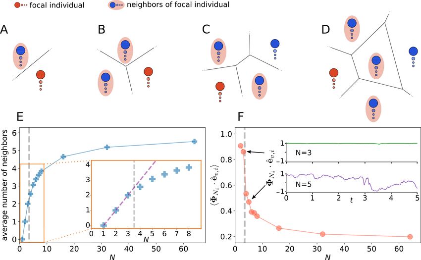
Figure 3: Influence of preferred speed and speed variability on polarization and speed-polarization coupling.
The preferred speed v0 and the speed relaxation strength β both affect the individual speed (A) and modulation of
either of these parameters may induce orientational order marked by a high polarization Φ (B). The transition to order
can be understood by a local coupling between the local average speed hviR and the local polarization ΦR , which we
quantified via their correlation Corr(hviR , ΦR ) (C). The local averages consider all individuals within a circle of
radius R = 3 around a focal one. Note that hviR is not the local group velocity (where a positive correlation with order
is trivial) but the local average of the individual speed magnitudes. The specific dependence between local speed and
order for three specific parameter choices (marked by square, circle and cross in C) is shown for the disordered state
(D), the phase transition region (E) and the ordered state (F). The parameters in the simulations are listed in Tab. S4.
reduce the average speed of individuals: A focal agent i aligns with the mean velocity of its neighbors hviNi . However,
for finite levels of directional fluctuations |hviNi | / vi , i.e. it will decelerate due to an effective social friction associated
with the alignment interaction [27]. The reduced speed allows a faster turning and consequently enhances the angular
noise and therefore disorder (Fig. 3B). Thus, in any collective system in which individuals align velocity vectors and
not only orientations, i.e. try to match not only the direction of motion but also their speed to the average perceived
movement of the local neighborhood, different collective states can emerge due to individuals in the corresponding
groups only differing in their speed variability with all other behavioral parameters being identical.
The dynamic speed variability (low β) has another highly robust emergent consequence. It allows agents of the same
collective to differ in their instantaneous speed and since higher speeds induce order, we observe correlations on the
local level between mean individual speed hviR and local polarization ΦR with R as the radius of the circle from which
the average is computed (Fig. 3C-F). Please note that as we consider individual speed, the above correlation is different
from the trivial correlation between local polarization and local group speed. The correlations between individual speed
and local polarization is always positive and largest at the transition between disorder and order. The latter is a signature
of second order phase transitions, where the susceptibility, i.e. the response to weak signals/fluctuations, is maximal. It
means that information encoded in speed is best translated to a directional response at the transition region, and vice
versa (likely to be beneficial in collective computation tasks).
The local coupling is an emergent consequence of the fundamental dependence of turning on speed. Thus, it is highly
robust and the qualitatively same non-linear functional form was observed in experiments (compare Fig. 3D-F with
Fig. 1 in [28]). Most importantly, it weakens with low speed variability (Fig. 3C) and does not exist for fixed speed
models.
8J UNE 18, 2021
Figure 4: Variable speed affects collective behavior in different states. Polarization Φ(A), the susceptibility χ (inset
A), the individual speed hsi (B), the area of the convex hull (C) and the nearest neighbor distance N N D (inset C) are
shown in dependence on the velocity alignment strength µalg . Black crosses (B, C) mark the peak of the susceptibility,
i.e. the location of the phase transition. The lines are color coded according to the speed relaxation strength as indicated
at the colorbar, i.e. β ∈ {1, 2, 4, 8, 16, 32, 64}.
3.2.2 Group structure and speed
We have demonstrated above that the preferred speed and its variability can induce an order-disorder transition. Now,
we keep the preferred speed fixed at v0 = 1 and change the alignment strength µalg . By repeating this for different
speed relaxation strength β we investigate how the collective behaves in the ordered and disordered state (controlled by
µalg ) depending on how variable the speed is.
The higher the speed variability of individuals, the larger alignment strengths are necessary for the collective to reach the
ordered state (Fig. 4A). The shift of the phase transition is more clearly depicted by shifting peaks of the susceptibility
χ = N (hΦ2 i − hΦi2 ) (fluctuations of the polarization, Fig. 4A inset).
The collective phase transition impacts the individual dynamics as well. The mean individual speed hsi shows a distinct
minimum at the transition which vanishes for low speed relaxation strength β = 1 (Fig. 4B). The minimum in speed
is related to the velocity alignment where a focal agent adjusts its velocity vi to the average velocity vector of its
neighbors hviNi . In the disordered state hviNi ≈ 0, i.e. the alignment interaction induces an effective social friction
−µalg vi and thus slows the focal agent down [27]. It changes at the disorder-order transition where the neighborhood
of each agent becomes increasingly polarized with increasing alignment strength. However, since there is always noise
on the heading direction |hviNi | < v0 , even in the strongly ordered state the individual speed is below the preferred
speed v0 .
A very general qualitative change from fixed to variable speed can be observed with respect to group structure close to
the phase transition. The area of the convex hull of the collective is maximal at the transition for fixed speeds. This
maximum becomes less pronounced and finally vanishes with increasing speed variability (lower speed relaxation
strength β, Fig. 4C). The same holds for the nearest neighbor distance (Fig. 4C inset). At the transition the directional
correlation of the agents is maximal (i.e. susceptibility peaks, Fig. 4A inset) and the directional fluctuations cause
subgroups of the collective to head in different directions, leading to an expansion of the collective [22]. This expansion
weakens with increasing speed variability because the distance regulating force can now lower the speed from a
subgroup if it moves away from the shoal, effectively inhibiting expansion.
3.2.3 Group size dependent effects
Group size is among the most biologically most important and experimentally most easily controllable parameters in
the context of flocking and schooling. Thus, we investigate in this last part how group and individual measures change
with group size N .
9J UNE 18, 2021
Figure 5: Group size effects depend on speed variability. The polarization Φ (A), the susceptibility χ (B) and the
mean individual speed hvi (C) are shown for different speed relaxation strength β and group sizes N .
For high speed variability, i.e. low speed relaxation strength β, polarization decreases with increasing groups size and
we expect Φ → 0 for even larger N (Fig. 5A). For low speed variability (large β), the polarization remains high Φ . 1
independent on N . Note that only in a narrow range close to the transition (marked by a large susceptibility, Fig. 5B),
the polarization saturates to intermediate values for large groups.
With group size being a key parameter, the question regarding existence of a threshold size, where the system’s behavior
changes qualitatively, is of particularly relevance. Our results show that for agents with high speed variability (low β),
the mean individual speed hvi undergoes a sudden change at N = 3 (Fig. 5C). Until N = 3 the individual speed hvi is
larger than v0 and saturates towards v0 with decreasing speed variability (increasing β). The reason for hvi > v0 is that
the speed distribution of individuals is asymmetric, with a long-tail at large speeds but cutoff at low speeds at v = 0
(Fig. 2, A-D), i.e. a maximum of the distribution is at v = v0 but the mean is larger. For larger groups with N ≥ 4, the
speed is lower than the preferred speed but saturates also to v0 in the fixed speed limit (β → ∞).
This abrupt change can be understood through the interplay of individual dynamics and fundamental property of the
interaction network: (i) A focal agent decelerates stronger the more its heading deviates from the average polarization
of its neighborhood, i.e. dvi /dt ∝ ΦNi · êv,i − 1 (derived in SI Sec. III). (ii) For Voronoi-type interaction, for
group size N ≤ 3, we have an all-to-all interaction network, which is not the case for N > 3. The second point is
illustrated in Fig. 6A-D, where only for N > 3 a set Di of agents disconnected from the focal agent i can exists, i.e.
Di = A \ (Ni ∪ {i}) 6= ∅ for N > 3 with A as the set of all agents of the group. We confirmed this by computing the
average number of neighbors during the simulations (Fig. 6E).
In summary, for N ≤ 3 we have an all-to-all coupling, thus all agents receive the same social input, whereas for N > 3,
centrally located individuals receive ”independent” social inputs from different neighbors on different sides, which are
not neighbors themselves, i.e. are not directly interacting. Thus, for N > 3 the centrally located individuals seek a
compromise between two independent sources of information. As a consequence, the neighborhood of a focal agent
located on the edge and the edge-agent itself, agree less in velocity. This results in slowing down the focal edge-agent,
which in turn feeds back on the group behavior. To support this explanation we computed the vector product ΦNi · êv,i
which shows a sudden decrease from N = 3 to N = 4 (Fig. 6F).
4 Discussion
We have shown experimental evidence of speed variability in fish and that inertia together with rotational friction
explain the reduced turning ability at larger speeds. With our model that incorporates both, we explored the effect of
speed variability on the emergent collective behavior.
10J UNE 18, 2021
Figure 6: Qualitative topological change with group size. A-D: illustrations of typical spatial constellations for
different group sizes. The focal (red) agent and it’s neighbors (blue in red ellipse) and for groups N ≥ 4 also agents
that are not connected to the focal agent (blue) are shown. E: average Voronoi neighbor number for different group
sizes. The dashed purple line (inset E) marks the numbers of neighbors of a fully connected group. F: average vector
product of neighborhood polarization vector ΦNi and the heading direction êv,i of the focal agent i. The time series of
the vector product (inset F) reveals a distinct difference between groups of N = 3 and N ≥ 4.
Naturally, the decrease of turning rate at higher individual speeds will inhibit individual directional noise, and thus
facilitate stronger group polarization. Note, that this effect of speed-dependent turning rate comes on top of previously
identified positive impact of higher speeds on group order [3]. However, not only differences in (average) speed itself,
but also differences in individual speed variability for the same average individual speed can result in differences in
polarization between groups. We find that the local speed correlates strongest with the local polarization at the order-
disorder transition, i.e. fixed speed models that investigate this prominent transition miss one of its crucial components.
For example, fixed speed models show at this transition a strong feedback between the maximum susceptibility to
perturbations and the self-organized group structure [22], which becomes less pronounced and eventually vanishes for
large enough speed variability. Finally, we unveil a sudden decrease in individual average speed at a threshold group
size only present at sufficiently high speed variability, which intrinsically linked to the fundamental structure of the
interaction network.
The transition from ordered to disordered motion with speed was reported in experiments [32, 25, 28]. However,
corresponding models incorporating a dependence of turning rate on speed were based on fitting of experimental data
and not on the fundamental physics of inertia and rotational friction (see e.g. [25, 28]). This order-disorder transition
induced by speed might enhance collective computation, as collective gradient sensing reported in golden shiners [1].
If a model mimics the reported increased/decreased speed for undesired/desired environmental cues (light intensity),
a variable speed model that correctly accounts for inertia could enhance the tendency of the collective to stay in the
desired environment because there it would be disordered, further decreasing group speed.
11J UNE 18, 2021
To elaborate the connection to collective computation we stress that the reported maximum of the local correlation
between polarization and speed at the disorder-order transition supports the criticality hypothesis [47, 48]. More
specifically, it suggests that at the transition, also referred to as the critical point, information encoded in the speed
is linked strongest to directional information, i.e. the individuals within the group show the strongest response to
directional information via speed adaptations and vise versa. However, we have also shown that spatial group properties
show distinct extrema at the transition for fixed-speed models, which are weakened or can even vanish with increasing
speed variability. This may have important implications regarding observations and conclusions drawn based on
investigation of fixed speed models and highlights the complexity of the transition region [22].
The distance regulating force, combining attraction and repulsion is required to obtain a cohesive shoal, and we used
here a simple, yet generic form, of this interaction. For the alignment interaction experimental evidence is species
[2, 45, 30] and group size dependent [25, 49, 31] but the chosen form is as general as possible. The individual processing
of velocity information can be even more elaborate than just taking into account the velocity differences of all neighbors.
An extension was studied by Lemasson et al. [50] where a focal agent only processes information of those neighbors
that move significantly faster compared to its total neighborhood. However, as long as the velocity alignment force acts
also on the speed of the agent our qualitative results are expected to hold.
Specific experimental data can be mimicked by a multitude of models which differ strongly in their microscopic
interactions [51, 52, 24, 31]. However, those models are most often fit to a specific experimental setup, i.e. to a certain
group size, tank size and depth, and need to be recalibrated if the setup changes [25]. Recently [26] suggested that
the experimentally observed decrease in polarization with larger groups is an emergent property of a model with only
pairwise interactions. However, in our model with a low speed relaxation strength β, we observe the same functional
dependence of polarization on group size. Linking our results again to criticality: only at the disorder-order transition
does the polarization saturates for large groups to intermediate values.
The reported sudden speed decrease in our variable speed model at a critical group size of N = 3, linked to a transition
from an all-to-all network to a distributed spatial network, might offer alternative means to test hypotheses about the
underlying interaction network in real animal groups [18, 44]. In our model Voronoi-interactions cause the specific size
threshold at N = 3, but for example for k-nearest neighbor interaction a group is all-to-all connected up to a threshold
size directly set by k, i.e. for N < k. However, in order to observe this qualitative change the neighbors have to align
their velocity vectors [37, 53], i.e. also match their speeds instead of only matching their movement direction. There
might be also other limitation to this approach, however the emergent speed-structure coupling clearly shows how
taking into account variable speed may introduce novel effects at the group level via the self-organized interplay of
speed and orientation dynamics and social interactions. Thus, we conclude that extreme caution should be taken when
drawing strong conclusions on collective behavior of animal groups based on agent-based models with fixed speed.
Conflict of Interest Statement
The authors declare that the research was conducted in the absence of any commercial or financial relationships that
could be construed as a potential conflict of interest.
Author Contributions
PPK, LGN and PR designed the analysis and wrote the paper. TL and DB provided the experimental data and
commented on the draft.
12J UNE 18, 2021
Funding
We received financial support by the DFG (German Research Foundation) under BI 1828/2-1, RO 4766/2-1, LA
3534/1-1 and under the Germany’s Excellence Strategy – EXC 2002/1 “Science of Intelligence” – project number
390523135.
Acknowledgments
We are thankful to Jens Krause for stimulating discussions.
Supplemental Data
Data Availability Statement
The experimental data sets are available in previous articles [36, 38, 33]. The code to run the agent-based model is
available at github (https://github.com/PaPeK/swarm-variable-speed).
References
[1] Andrew Berdahl, Colin J Torney, Christos C Ioannou, Jolyon J Faria, and Iain D Couzin. Emergent Sensing of
Complex Environments by Mobile Animal Groups. Science, 339(6119):574–576, feb 2013.
[2] Yael Katz, Kolbjørn Tunstrøm, Christos C. Ioannou, Cristián Huepe, and Iain D. Couzin. Inferring the structure
and dynamics of interactions in schooling fish. Proceedings of the National Academy of Sciences of the United
States of America, 108(46):18720–18725, 2011.
[3] Jolle W. Jolles, Neeltje J. Boogert, Vivek H. Sridhar, Iain D. Couzin, and Andrea Manica. Consistent Individual
Differences Drive Collective Behavior and Group Functioning of Schooling Fish. Current Biology, 27(18):2862–
2868.e7, sep 2017.
[4] A. J. W. Ward, James E. Herbert-Read, D. J. T. Sumpter, and Jens Krause. Fast and accurate decisions through
collective vigilance in fish shoals. Proceedings of the National Academy of Sciences, 108(6):2312–2315, feb 2011.
[5] Jens Krause and Jean-Guy J. Godin. Shoal Choice in the Banded Killifish (Fundulus diaphanus, Teleostei,
Cyprinodontidae): Effects of Predation Risk, Fish Size, Species Composition and Size of Shoalsnkkk. Ethology,
98(2):128–136, apr 1994.
[6] Colin J. Torney, Tommaso Lorenzi, Iain D. Couzin, and Simon A. Levin. Social information use and the evolution
of unresponsiveness in collective systems. Journal of The Royal Society Interface, 12(103):20140893, feb 2015.
[7] José A Carrillo, Massimo Fornasier, Giuseppe Toscani, and Francesco Vecil. Particle, kinetic, and hydrodynamic
models of swarming. In Mathematical modeling of collective behavior in socio-economic and life sciences, pages
297–336. Springer, 2010.
[8] Thomas Ihle. Kinetic theory of flocking: Derivation of hydrodynamic equations. Physical Review E, 83(3):030901,
2011.
[9] Jorge Hidalgo, Jacopo Grilli, Samir Suweis, Miguel A. Munoz, Jayanth R. Banavar, and Amos Maritan.
Information-based fitness and the emergence of criticality in living systems. Proceedings of the National
Academy of Sciences, 111(28):10095–10100, jul 2014.
[10] Randal S. Olson, Arend Hintze, Fred C. Dyer, David B. Knoester, and Christoph Adami. Predator confusion is
sufficient to evolve swarming behaviour. Journal of The Royal Society Interface, 10(85):20130305, aug 2013.
13J UNE 18, 2021
[11] Liang Li, Máté Nagy, Jacob M. Graving, Joseph Bak-Coleman, Guangming Xie, and Iain D. Couzin. Vortex phase
matching as a strategy for schooling in robots and in fish. Nature Communications, 11(1):5408, dec 2020.
[12] Tim Landgraf, David Bierbach, Hai Nguyen, Nadine Muggelberg, Pawel Romanczuk, and Jens Krause. RoboFish:
increased acceptance of interactive robotic fish with realistic eyes and natural motion patterns by live Trinidadian
guppies. Bioinspiration & Biomimetics, 11(1):015001, jan 2016.
[13] Tamás Vicsek and Anna Zafeiris. Collective motion. Physics reports, 517(3-4):71–140, 2012.
[14] A. Cavagna, A. Cimarelli, I. Giardina, G. Parisi, R. Santagati, F. Stefanini, and M. Viale. Scale-free correlations in
starling flocks. Proceedings of the National Academy of Sciences, 107(26):11865–11870, 2010.
[15] Ofer Feinerman, Itai Pinkoviezky, Aviram Gelblum, Ehud Fonio, and Nir S. Gov. The physics of cooperative
transport in groups of ants. Nature Physics, 14(7):1–11, jul 2018.
[16] Hugues Chaté, Francesco Ginelli, Guillaume Grégoire, Fernando Peruani, and Franck Raynaud. Modeling
collective motion: variations on the vicsek model. The European Physical Journal B, 64(3):451–456, 2008.
[17] Fernando Peruani, Tobias Klauss, Andreas Deutsch, and Anja Voss-Boehme. Traffic jams, gliders, and bands in
the quest for collective motion of self-propelled particles. Physical Review Letters, 106(12):128101, 2011.
[18] M Ballerini, N Cabibbo, R Candelier, A Cavagna, E Cisbani, I Giardina, V Lecomte, A Orlandi, G Parisi,
A Procaccini, M Viale, and V Zdravkovic. Interaction ruling animal collective behavior depends on topological
rather than metric distance: Evidence from a field study. Proceedings of the National Academy of Sciences,
105(4):1232–1237, 2008.
[19] Ariana Strandburg-Peshkin, Danai Papageorgiou, Margaret C. Crofoot, and Damien R. Farine. Inferring influence
and leadership in moving animal groups. Philosophical Transactions of the Royal Society B: Biological Sciences,
373(1746), 2018.
[20] Hangjian Ling, Guillam E Mclvor, Joseph Westley, Kasper van der Vaart, Richard T Vaughan, Alex Thornton, and
Nicholas T Ouellette. Behavioural plasticity and the transition to order in jackdaw flocks. Nature communications,
10(1):1–7, 2019.
[21] Tamás Vicsek, András Czirók, Eshel Ben-Jacob, Inon Cohen, and Ofer Shochet. Novel type of phase transition in
a system of self-driven particles. Physical review letters, 75(6):1226, 1995.
[22] Pascal P. Klamser and Pawel Romanczuk. Collective predator evasion: Putting the criticality hypothesis to the test.
PLOS Computational Biology, 17:1–21, 03 2021.
[23] Jolle W. Jolles, Andrew J. King, and Shaun S. Killen. The Role of Individual Heterogeneity in Collective Animal
Behaviour. Trends in Ecology & Evolution, 35(3):278–291, mar 2020.
[24] Iain D. Couzin, Jens Krause, Richard James, Graeme D. Ruxton, and Nigel R. Franks. Collective memory and
spatial sorting in animal groups. Journal of Theoretical Biology, 218(1):1–11, 2002.
[25] Jacques Gautrais, Francesco Ginelli, Richard Fournier, Stéphane Blanco, Marc Soria, Hugues Chaté, and Guy
Theraulaz. Deciphering interactions in moving animal groups. PLOS Computational Biology, 8(9):1–11, 09 2012.
[26] Jitesh Jhawar, Richard G. Morris, U. R. Amith-Kumar, M. Danny Raj, Tim Rogers, Harikrishnan Rajendran, and
Vishwesha Guttal. Noise-induced schooling of fish. Nature Physics, 16, Apr 2020.
[27] R Großmann, L Schimansky-Geier, and P Romanczuk. Active brownian particles with velocity-alignment and
active fluctuations. New Journal of Physics, 14(7):073033, jul 2012.
[28] Shradha Mishra, Kolbjørn Tunstrøm, Iain D. Couzin, and Cristián Huepe. Collective dynamics of self-propelled
particles with variable speed. Phys. Rev. E, 86:011901, Jul 2012.
[29] Roy Harpaz, Gašper Tkačik, and Elad Schneidman. Discrete modes of social information processing predict
individual behavior of fish in a group. Proceedings of the National Academy of Sciences, 114(38):10149–10154,
sep 2017.
14J UNE 18, 2021
[30] Daniel S Calovi, Alexandra Litchinko, Valentin Lecheval, Ugo Lopez, Alfonso Pérez Escudero, Hugues Chaté,
Clément Sire, and Guy Theraulaz. Disentangling and modeling interactions in fish with burst-and-coast swimming
reveal distinct alignment and attraction behaviors. PLOS Computational Biology, 14(1):e1005933, jan 2018.
[31] Valerio Sbragaglia, Pascal P Klamser, Pawel Romanczuk, and Robert Arlinghaus. Unexpected harvesting-induced
evolution of collective behavior in a fish. In review at The American Naturalist, 2020.
[32] Maud I. A. Kent, Ryan Lukeman, Joseph T. Lizier, and Ashley J. W. Ward. Speed-mediated properties of schooling.
Royal Society Open Science, 6(2):181482, feb 2019.
[33] Jolle W. Jolles, Nils Weimar, Tim Landgraf, Pawel Romanczuk, Jens Krause, and David Bierbach. Group-
level patterns emerge from individual speed as revealed by an extremely social robotic fish. Biology Letters,
16(9):20200436, 2020.
[34] Daniel S. Calovi, Ugo Lopez, Sandrine Ngo, Clément Sire, Hugues Chaté, and Guy Theraulaz. Swarming,
schooling, milling: phase diagram of a data-driven fish school model. New Journal of Physics, 16(1):015026, jan
2014.
[35] Denis Réale, Simon M. Reader, Daniel Sol, Peter T. McDougall, and Niels J. Dingemanse. Integrating animal
temperament within ecology and evolution. Biological Reviews, 82(2):291–318, may 2007.
[36] David Bierbach, Kate L. Laskowski, and Max Wolf. Behavioural individuality in clonal fish arises despite
near-identical rearing conditions. Nature Communications, 8, 2017.
[37] J. E. Herbert-Read, S. Krause, L. J. Morrell, T. M. Schaerf, J. Krause, and A. J. W. Ward. The role of individuality
in collective group movement. Proceedings of the Royal Society B: Biological Sciences, 280(1752):20122564, feb
2013.
[38] Carolina Doran, David Bierbach, and Kate L. Laskowski. Familiarity increases aggressiveness among clonal fish.
Animal Behaviour, 148:153–159, 2019.
[39] Hauke J. Mönck, Andreas Jörg, Tobias von Falkenhausen, Julian Tanke, Benjamin Wild, David Dormagen, Jonas
Piotrowski, Claudia Winklmayr, David Bierbach, and Tim Landgraf. BioTracker: An open-source computer
vision framework for visual animal tracking. arXiv, 2018.
[40] Pawel Romanczuk, Markus Bär, Werner Ebeling, Benjamin Lindner, and Lutz Schimansky-Geier. Active brownian
particles. The European Physical Journal Special Topics, 202(1):1–162, 2012.
[41] Pawel Romanczuk. Active Motion and Swarming. From Individual to Collective Dynamics. PhD thesis, Humboldt
University of Berlin, 2011.
[42] H. Akaike. A new look at the statistical model identification. IEEE Transactions on Automatic Control, 19(6):716–
723, 1974.
[43] Gideon Schwarz. Estimating the Dimension of a Model. The Annals of Statistics, 6(2):461 – 464, 1978.
[44] Ariana Strandburg-Peshkin, Colin R Twomey, Nikolai WF Bode, Albert B Kao, Yael Katz, Christos C Ioannou,
Sara B Rosenthal, Colin J Torney, Hai Shan Wu, Simon A Levin, et al. Visual sensory networks and effective
information transfer in animal groups. Current Biology, 23(17):R709–R711, 2013.
[45] James E. Herbert-Read, Andrea Perna, Richard P. Mann, Timothy M. Schaerf, David J.T. Sumpter, and Ashley J.W.
Ward. Inferring the rules of interaction of shoaling fish. Proceedings of the National Academy of Sciences of the
United States of America, 108(46):18726–18731, nov 2011.
[46] Fernando Peruani and Luis G Morelli. Self-propelled particles with fluctuating speed and direction of motion in
two dimensions. Physical review letters, 99(1):010602, 2007.
[47] Thierry Mora and William Bialek. Are Biological Systems Poised at Criticality? Journal of Statistical Physics,
144(2):268–302, 2011.
15J UNE 18, 2021
[48] Miguel A. Muñoz. Colloquium: Criticality and dynamical scaling in living systems. Reviews of Modern Physics,
90(3):31001, 2018.
[49] Adam K. Zienkiewicz, Fabrizio Ladu, David A.W. Barton, Maurizio Porfiri, and Mario Di Bernardo. Data-driven
modelling of social forces and collective behaviour in zebrafish. Journal of Theoretical Biology, 443:39–51, apr
2018.
[50] Bertrand H Lemasson, James J Anderson, and R A Goodwin. Motion-guided attention promotes adaptive commu-
nications during social navigation. Proceedings. Biological sciences / The Royal Society, 280(1754):20122003,
2013.
[51] Renaud Bastien and Pawel Romanczuk. A model of collective behavior based purely on vision. Sci. Adv.,
6(6):1–10, 2020.
[52] Pawel Romanczuk, Iain D. Couzin, and Lutz Schimansky-Geier. Collective Motion due to Individual Escape and
Pursuit Response. Physical Review Letters, 102(1):010602, jan 2009.
[53] James E. Herbert-Read, Emil Rosén, Alex Szorkovszky, Christos C. Ioannou, Björn Rogell, Andrea Perna,
Indar W. Ramnarine, Alexander Kotrschal, Niclas Kolm, Jens Krause, and David J. T. Sumpter. How predation
shapes the social interaction rules of shoaling fish. Proceedings of the Royal Society B: Biological Sciences,
284(1861):20171126, aug 2017.
16J UNE 18, 2021
SI Appendix
Supplementary Information
“Impact of Variable Speed on Collective Movement of Animal
Groups”
Pascal P. Klamser1,2 , Luis Gómez Nava1,3 , Tim Landgraf3,4 , Jolle W. Jolles,5 , David Bierbach,3,6,7 , Pawel
Romanczuk1,2,3,*
1 Institute for Theoretical Biology, Department of Biology, Humboldt Universität zu Berlin, Berlin, Germany.
2 Bernstein Center for Computational Neuroscience, 10115 Berlin, Germany.
3 Cluster of Excellence, Science of Intelligence, Technische Universität Berlin, Berlin, Germany,
4 Department of Mathematics and Computer Science, Freie Universität Berlin, Berlin, Germany.
5 Center for Ecological Research and Forestry Applications (CREAF), Campus de Bellaterra (UAB), Barcelona, Spain.
6 Department of Biology and Ecology of Fishes, Leibniz-Institute of Freshwater Ecology and Inland Fisheries, Berlin,
Germany.
7 Faculty of Life Sciences, Albrecht Daniel Thaer-Institute of Agricultural and Horticultural Sciences, Humboldt
Universität zu Berlin, Berlin, Germany.
I Details on experimental setups
The experimental data presented in this article was published in Jolles et al. [33] (guppies and RoboFish), Bierbach et al.
[36] (single mollies) and Doran et al. [38] (groups of mollies). In the following we summarize the setups of each study.
I.1 Individual guppy and RoboFish trajectories
For this experiments, only adult female individuals (Trinidadian guppies) were used, which have a standard body length
of (31.7 ± 0.8 mm). The single individual trajectories were obtained by putting single fish in a 88cm × 88cm white
glass tank. The behavior was recorded over an observation period of 10 minutes using an acquisition frame rate of 30
FPS. The videos were then processed using the software BioTracker [39] to obtain the tracking of each fish.
For the RoboFish trials, a three-dimensional-printed fish replica was used. This replica was connected to a two-wheeled
robot below the tank (see Fig. S1 of the SI in [33]). The robot was controlled by a closed-loop system whereby the
movements of the fish were identified and fed back to the robot control. The robot was able to adjust its position and
direction of motion to mimic natural responses. The robot’s behavior was based on the zonal model explained in [24].
For more details on the acquisition of the experimental data, see [33].
I.2 Mollies trajectories: single individual experiments
The experiments were performed using clonal Amazon mollies using a open field circular tank (48.5cm of diameter)
made of white plastic. Single fish were introduced and observed for periods of 5 minutes. Its behavior and motion
were recorded and its positions were acquired with the tracking software Ethovision Version 10.1 (Noldus Information
Technologies Inc.). For more details on the data acquisition, see [36].
I.3 Mollies trajectories: group experiments
For these experiments, 32 fish were used. They were assembled in groups of 4 individuals, leading to 8 groups in
total. The fish were adult sized-matched mollies of a standard body lenght of (6.14 ± 0.76 cm). The experiments were
1J UNE 18, 2021
RoboFish Guppy Molly Mollies(N=4) Model
F α F α F α F α F α
dϕ
dt = F/v 0.1 0.1 0.45 0.2 6.2
dϕ
dt = F/(v + α) 4.1 0.13 10.6 0.17 4.74 0.16 3.03 0.4 29.1 0.99
Table S3: Statistical model parameters. Fitting parameters for the fits displayed in Fig. 2.
standard Fig. 2 Fig. 3 Fig. 4 Fig. 5
preferred speed v0 1 [0.1, 4] 2
speed relaxation β 0.2 [0.25, 10.76] [1, 64] [0.025, 10.76]
single
turn friction α 1 0.1
angular noise Dϕ 1
velocity noise Dv 0.4
group size N 400 1
collective
alignment strength µalg 2 - [0, 5.9]
distance strength µd 2 -
distance slope md 2 -
preferred distance rd 1 -
Table S4: Parameters used in simulations. The different columns after the ”standard” column list parameters which
differ from standard parameters for the simulations represented by the respective figures.
performed in a 60cm × 30cm arena. The groups were left unperturbed for periods of 5 minutes, in which their behavior
was recorded using an acquisition frame rate of 30 FPS. The positions of the individuals were obtained from the videos
using the tracking software Ethovision XT12 (Noldus Information Technology, Inc.). For more details on the data
acquisition, see [38].
II Derivation of turning dependence on speed
Here we show in detail how to derive the dynamics of speed and turning angle from the change in velocity:
dvi 1
= Fi (S1)
dt m
with vi as the velocity vector of the object, m its mass and Fi as the force acting on it. The velocity vector can be
expressed via the speed vi and the heading angle ϕi to vi = vi [cos ϕi , sin ϕi ]T = vi êv,i . We can reformulate the
velocity dynamics by the speed and heading angle dynamics to
dvi d dvi dϕi dêv,i
= (vi êv,i ) = êv,i + vi (S2)
dt dt dt dt dϕi
" #
dvi dϕi − sin ϕi
= êv,i + vi (S3)
dt dt cos ϕi
dvi dϕi
= êv,i + êϕ,i vi . (S4)
dt dt
T T
where êv,i = cos ϕi (t), sin ϕi (t) and êϕ,i = − sin ϕi (t), cos ϕi (t) are unitary vectors in the particle’s heading
and turning directions respectively. Thus, the change in speed and heading angle is
2You can also read