Indian Association of Alternative
    Investment Funds (IAAIF)
←
→
Page content transcription
If your browser does not render page correctly, please read the page content below
Indian Association of Alternative
Investment Funds (IAAIF)
Portfolio Construction with
 Alternative Investments
    Rohan Misra, CFA, FRM
        Partner & CEO

    Transparency. Safety. Performance.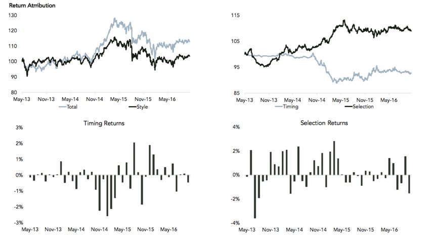
AGENDA
PART 1:
PORTFOLIO CREATION
           FINDING THE EQUILIBRIUM
1. ASSET ALLOCATION
2. ACTIVE VS PASSIVE BALANCE
3. MANAGER/FUND SELECTION
PART 2:
PORTFOLIO PERFORMANCE EVALUATION
AND REBALANCING
                                     3
Part 1: Portfolio Creation
Finding the equilibrium…

         …By mixing a number of poorly
         correlated assets, and -

         •   Maximize target return for a given level
             of risk

         •   Minimize risk for a targeted level of
             return

                                                        5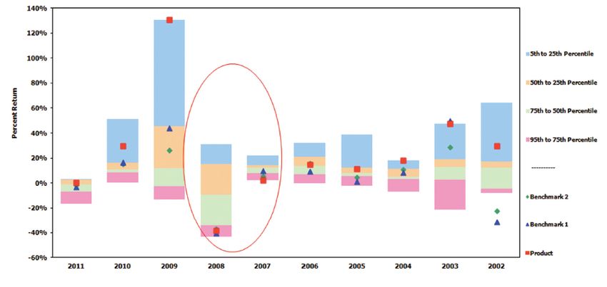
2 ways to construct portfolios
  Bottom Up                                    Top down

• Used by private           Asset THE EQUILIBRIUM
                      FINDING          • Favoured by
  investors              Allocation      professional
                                          investors
• Adhoc –
  objectives and                       • Begins by exploring
                         Active Vs
  risk not factored                      investment risk
                        Passive Mix
• Susceptible to                       • Creates a
  “buy high sell                         framework to
  low” behaviour      Manager/Fund       decide investments
                        Selection        based on investor’s
                                         objectives
                                                          6
Setting objectives
         Return             ILLUSTRATIVE EXAMPLE
                            Return Target:
       Typical Objectives:
       • Maximize return for5%aplus  inflation
                                 given level of;risk
                                                 after fees
       • Minimize risk for aRisk Budget
                             targeted     andofRisk
                                       level        Definition:
                                                return
 Risk              Time     Max loss 20%
Budget                      Time Horizon :
                            5 years
Examples of other considerations
1. Interim/Terminal Goals: financing a second home purchase
2. Constraints: dedicated assets (residential home), asset class
   restrictions , short selling restrictions

                                                                   7
PART 1: PORTFOLIO
FINDING CREATION
THE EQUILIBRIUM
1. ASSET ALLOCATION
2. ACTIVE VS PASSIVE BALANCE
3. MANAGER/FUND SELECTION
8What is an asset allocation (AA)
Portfolio strategy that involves setting target allocations for
various asset classes and attempts to balance risk versus
reward, according to the investor’s risk budget, goals and time
horizon
Strategic Asset Allocation (SAA)
Driven by the long-term investment
objectives of the investor, with a
typical time frame of > 1Y
Tactical Asset Allocation (TAA)
Represents short-term tilts away from
the SAA that are driven by visible
opportunities and risks
9Why begin with AA?
Decomposition of Time-Series Total Return Variations
150
100
R square %
50
0
-50
BHB Equity Funds BHB Balanced HEI & IK Equity HEI & IK Balanced
Funds Funds Funds
Active Management Asset Allocation Policy
Market Movement Interaction Effect
BHB: Brinson, Hood, Beebower, Determinants of Portfolio performance, 1986
IK: Ibbotson & Kaplan, Does AA explain 40,90 or 100% of performance?, 2000
HEI: Henzel, Ezra, Ilkiw, The importance of the AA decision, 1991
10Choice of asset classes and their
mix is key
• For portfolios with market exposures, e.g. long only portfolios,
market movement and asset allocation policy mainly drive
return variability
• Market movement is a function of the chosen asset classes
• Asset allocation policy defines how we have mixed the chosen
asset classes
• Can we improve an asset allocation by including alternatives
like Hedge Funds, PE, Real Estate and Commodities??
11Asset class choices
Asset Class Proxy Index Currency Freq.
MSCI All Country World Net Total
Equities USD Monthly
Return Index
Bloomberg Barclays US Govt Total
Bonds USD Monthly
Return Index Unhedged USD
Commodities Bloomberg CMCI Total Return Index USD Monthly
HFRI Fund Of Hedge Funds
Hedge Funds USD Monthly
Composite Index
FTSE EPRA NARIET Developed Total
Real Estate USD Monthly
Return Index
Cambridge Associates US Private
Private Equity USD Quarterly
Equity Index
All indices are assumed for illustration purposes only, All data starting Jan-2000
12Summary statistics
Hedge Real Private
Equity Bonds Com
Funds Estate Equity
Ann. Return 3.5% 4.8% 6.4% 3.2% 9.5% 9.7%
Ann.
Volatility
16.0% 4.2% 16.2% 5.1% 19.1% 10.4%
Max
DrawDown
54.9% 4.6% 57.1% 22.2% 67.2% 25.2%
Return/
Volatility
0.22 1.16 0.40 0.64 0.50 1.01
Equity returns biased downwards as sample begins in Tech bubble, 13
Source: B&B AnalyticsRisk/Return Profiles
12.0%
PE
10.0% RE
8.0%
6.0% COM
Bonds
4.0% EQ
2.0% HF
0.0%
0.0% 5.0% 10.0% 15.0% 20.0% 25.0%
Note! : Profiles may be potentially biased due to the chosen sample since 2000
Source: B&B Analytics
14In-sample correlations
Hedge Real Private
Equity Bonds Com
Funds Estate Equity
Equity 1.00
Bonds -0.28 1.00
Com 0.56 -0.17 1.00
Hedge Funds 0.67 -0.13 0.58 1.00
Real Estate 0.80 -0.03 0.49 0.58 1.00
Private Equity 0.52 -0.29 0.35 0.41 0.40 1.00
Average
0.45 -0.18 0.36 0.42 0.45 0.28
Correlations
Source: B&B Analytics 15Impact of introducing Alts in a
50 Eq/50 bonds portfolio
45 Eq; 45 Eq; 45 Eq; 45 Eq;
50 Eq;
45 Bonds; 45 Bonds; 45 Bonds; 45 Bonds;
50 Bonds
10 Com 10 HF 10 RE 10 PE
Ann Return 3.9% 4.1% 3.8% 4.3% 4.4%
Volatility
7.7% 7.9% 7.3% 8.6% 7.2%
Ann.
Return/Vol 0.50 0.51 0.52 0.50 0.61
Max
30% 31% 29% 35% 29%
DrawDown
Returns adjusted to the vol level of 50 Eq / 50 Bonds Portoflio
Ann. Return 3.9% 4.0% 4.0% 3.9% 4.7%
Source: B&B Analytics, portfolios rebalanced monthly 16Data biases and other vagaries
common to alternatives
171. Survivorship bias
• Generally accepted notion: Indices, in particular hedge funds
ones, are distorted because ‘closed’ funds no longer
contribute – and remaining funds overstate the average
• Some nuanced studies look at reason for closure and find
the index understates actual performance
1. ‘Closures’ due to negative performance
2. ‘Closures’ to new investors due to strong performance
• Jury is still out there!
• Partial remedy – Use a Hedge Fund FoF Index
Returns 1Y 2Y 3Y
HFR Global Asset Wtd Composite 5.38% 8.31% 23.68%
HFR Fund of Funds Composite 4.16% 4.94% 17.25%
Source: B&B Analytics, HFRI 182. Smoothed & stale prices
• Esp. Relevant in the context of private equity and real estate
• Appraiser lacks confidence in the new evidence regarding
valuation - instead attaches too much weight on the most
recent empirical evidence
• Reported valuation lags true market valuation
• Positive serial correlation is introduced into returns
REDUCED VARIABILITY IN RETURNS
ACROSS TIME à UNDERSTATES RISK
NEEDS TO BE CORRECTED!
19Correcting for smoothed prices
• Vast body of academic work PE Beta P-Value Significant
exists Intercept 1.66 0.01 Yes
Lag1 0.32 0.00 Yes
• FGW 1993 is a one widely Lag2 0.17 0.09 No
adopted approach Lag3 -0.02 0.87 No
Lag4 0.02 0.80 No
• Removes serial autocorrelation
Beta P-Value Significant
to unsmooth the time series Intercept 2.04 0.00 Yes
• Time series is regressed against Lag1 0.38 0.00 Yes
lagged values to identify
r(t) = (r*(t) – 0.38r*(t-1))/w
statistically significant variables. US Private Equity* Volatility
• Unsmoothed series is obtained Smoothed Series 9.4%
Unsmoothed Series 15.7%
by removing these variables. Return 9.7%
Return/New Vol 0.62
*Source: Cambridge Associate, FGW : Fisher Geltner Webb
203. Non-normality and tail risk
• Most models assume that returns follow a “normal
distribution”
– Chance of move > 3 s.d. < 1/300
– Skewness = 0 ; return symmetry
– Kurtosis = 3
• In reality most asset classes exhibit negative skew and excess
kurtosis … i.e left tail risk
21This can be seen in our data
Hedge Real Private
Equity Bonds Com
Funds Estate Equity
Skewness -0.89 -0.20 -1.08 -1.15 -1.54 -0.57
Excess
Kurtosis
2.47 1.36 4.07 4.26 7.15 1.94
60
Real Estate Monthly Return Distribution
40
20
0
-30%
-28%
-25%
-23%
-20%
-18%
-15%
-13%
-10%
-8%
-5%
-3%
0%
3%
5%
8%
10%
13%
15%
18%
20%
23%
Directly incorporating volatility into models will underestimate risk and
lead to incorrect allocations
Source: B&B Analytics 22Adjusting for non-normality Two approaches: • Adjust the risk (std. deviation) of each asset class or investment to capture the higher moments of skewness and kurtosis before determining the optimal portfolio weights • Directly adjust the portfolio risk measure in the asset weighting process (i.e the optimization process) to incorporate the skewness and kurtosis of the portfolio for a given combination of weights • Second approach is convenient • Both approaches are appropriate only if the historical distribution appropriately captures higher moments Source: B&B Analytics 23
Portfolio Math

                 24
Recap: essence of portfolio
construction
• Maximize target return for a given level of risk
• Minimize risk for a targeted level of return
How to measure portfolio return and what is portfolio risk?
25Portfolio Return
Weighted average of the expected returns of portfolio components
Example: 2 asset class portfolio
26Variance as portfolio risk
• Not a simple weighted average of individual component risks.
• Requires an estimate of expected covariances between assets –
which first requires an estimate of the volatilities of all assets and
the correlations between them
or
Example: 2 asset class portfolio
(wi)’COV(wi)
Portfolio Volatility: √0.0504 = 22.4%
27VaR as a portfolio risk measure
• Investor’s don’t think in volatility terms!
• Focus is on downside risk
• Value at risk (VaR) focuses on the left tail of the return distribution
• Interpretation: 95% chance that portfolio loss will not exceed
X% over a given time horizon; 95% represents confidence
28Parametric VaR
• Assumes normal distribution – requires only mean and
standard deviation of returns to calculate VaR
• VaR (confidence) = Mean - Std. Dev * z
• ‘z’ is the normal z-score corresponding to the confidence level
(e.g. 1.65 for 95%, 1.96 for 99%)
• Simple but practically limited – does not include negative
skew and fat tails!
29Modified Parametric VaR
• Formulaic adjustment to parametric VaR for the empirically
observed skew and kurtosis of the portfolio return
distribution
• Somewhat better at capturing non-normality by transforming
the normal ‘z’ to a modified ‘Z’ incorporating higher moments
30Drawdown
• Max DD measures peak to trough loss – very conservative
• Difficult to implement in practice and needs to be simplified to an
either inception to date drawdowns or rolling drawdowns
31Optimal Portfolio Mix
Traditional Markowitz Approaches
based on Modern Portfolio Theory
32Optimization Setup
• Maximize Expected Portfolio Return subject to an absolute
constraint on risk 0% and < 35% (the latter to ensure
diversification)
33Expected Return adjustments
11.0%
10.0% PE
9.0%
8.0%
RE
7.0%
6.0%
5.0% EQ
COM
4.0%
Bonds HF
3.0%
2.0%
1.0%
0.0%
0.0% 5.0% 10.0% 15.0% 20.0% 25.0%
Adjustments done largely to reflect current thinking around capital market assumptions
Source: B&B Analytics, for illustrative purposes only
34Capital constraints (0,35%)
• Allocation to bonds and hedge funds increases as more conservative
approaches (VaR and mVaR) are used
100%
80% 35.0% 35.0% 35.0%
60% 19.5%
30.2% 22.6%
40%
35.0% 35.0%
20% 34.8%
10.5% 7.4%
0%
Mean Variance Mean VaR Mean mVaR
(Parametric) (Parametric) (Parametric)
Equity Bonds Commodities
Hedge Funds Real Estate Private Equity
35Portfolio Metrics
Mean Variance Mean VaR Mean mVaR
(Parametric) (Parametric) (Parametric)
Annualized Return 6.8% 6.1% 6.0%
Annualized Risk 10.0% 10.0% 10.0%
Return/Risk 0.68 0.61 0.60
Drawdown 30.3% 20.3% 19.2%
36Unconstrained efficient frontiers
12.0%
10.0%
8.0%
6.0%
4.0%
Return Vs Volatility (Parametric) Return Vs VaR (Parametric) Return Vs mVaR (Parametric)
37Optimal Portfolio Mix
Other Approaches
38Practical issues with traditional
approaches
Estimating many inputs for N asset classes
• N expected returns
• N expected volatilities
• N(N-1)/2 expected correlations
Capital Allocation Risk Allocation
Vs
Bonds Equities Bonds Equities
39Practical issues with traditional
approaches
Sensitivity of weights to changing equity return
assumptions
100%
18.3%
Unconstrained Weights
28.3%
80% 39.4%
51.1%
67.2% 67.2% 67.2% 67.2% 63.0% 31.5%
60% 30.5%
30.1%
40%
30.6%
32.0% 41.2% 50.3%
20% 32.8% 32.8% 32.8% 32.8% 30.5%
18.3%
0% 5.0%
7.00% 7.50% 8.00% 8.50% 9.00% 9.50% 10.00% 10.50% 11.00%
Equity Return Assumption
Equity Bonds Commodities Hedge Funds Real Estate Private Equity
40Risk Parity
• Lets throw some darts!
• Risk driven approaches – expected
returns not required to be estimated
• Based on premise that a range of
outcomes (risk) is easier to estimate
than the outcome (return)
• Optimize capital weights so that “risk contributions” of all asset classes
are equal
• Risk Contribution (RC) of asset i = W(i) X Std. Dev(p) X Beta (i,p)
• If an asset’s weight = 20%, its beta with portfolio = 2 , then assuming
portolio vol = 10%, the RC = 4% => or 40% of risk comes from the asset
41Risk Parity
Asset Allocation Risk Contribution
7.2% 5.8%
4.7%
20.0% 20.0%
Equity
Bonds
18.0% Commodities 20.0% 20.0%
Hedge Funds
57.5%
Real Estate
6.8% 20.0% 20.0%
Private Equity
Portfolio Evolution
300
Risk Parity
Annualized Return 4.1%
200
Annualized Risk 4.1%
100 Return/Risk 0.99
2000 2003 2006 2009 2012 2015
Risk Parity Drawdown 12.8%
Criticism: Too much weight to fixed income, requires leverage to scale to traditional
42
portfolio risk budgetsRisk Budgeting
• Optimize capital weights so that ”risk contribution” of each
asset class falls within the max risk contribution allocated to it
• This involves setting risk contribution budgets e.g. RC(1) = X ,
RC(2) = Y …
• Sum [ RC(i) ] = Portfolio Standard Deviation
• Robust alternative to using expected returns -> Increase risk
budgets if view on asset class is positive , decrease risk budget
if the view is negative
43PART 1: PORTFOLIO
FINDING CREATION
THE EQUILIBRIUM
1. ASSET ALLOCATION
2. ACTIVE VS PASSIVE BALANCE
3. MANAGER/FUND SELECTION
44Are alternative betas investable?
Asset Class Developed Markets India
Thousands of ETFs available by Few ETFs, but many MFs to
Equities (EQ)
region, market, sector and style choose from
Fixed Income Large number of ETFs available by ETFs practically non-existent;
(FI) FX, Duration, Rating, Risk country but several MFs to choose from
Commodities Many ETF and ETN options
Few, largely limited to Gold
(COM) on most commodities
1st REIT expected in 2017; RE
Real Estate (RE) REIT & CEF/FoF options available
PE Funds existing
Hedge Funds Several HF Index replication & FoF PMS, AIF funds, Largely single
(HF) available managers
Private Equity
Diversified FoF options available Largely single managers
(PE)
45Unfortunately not
• Traditional betas (EQ,FI,COM) cheaply available
• Alt managers (HF,PE,RE) mainly seek to deliver alpha
• Alt betas not easily available (at least for HF, PE, RE)
• High dispersion of Alt returns makes it difficult to replicate
benchmarks, FoF investment route solves this problem only
partially
Solution: Treat Alts (esp HF,PE,RE) as a part of an active
management mandate
46Core & Satellite Approach
Satellite
• Core: long-term, low-cost investments
including ETFs, MFs etc seeking market returns Core
(EQ and FI and possibly COM betas)
• Satellite: actively managed alpha producing
investments seeking to deliver absolute return
(HF,PE,RE) Asset Passive Active
• A best of both (active & passive) worlds Class (Core) (Satellite)
approach EQ ✔ ✔
• Optimize costs (inexpensive core) FI ✔ ✔
• Potential to outperform the asset COM ✔ ✔
allocation RE ✔
• Diversify risk through greater number of HF ✔
holdings PE ✔
47But this should be consistent
with Asset Allocation
1. E[RC(core + satellite)] = E[R(asset class in SAA)]
Where E[R] is expected return and E[RC] is expected risk
contribution.
Nice in theory, difficult to achieve in practice!
48PART 1: PORTFOLIO
FINDING CREATION
THE EQUILIBRIUM
1. ASSET ALLOCATION
2. ACTIVE VS PASSIVE BALANCE
3. INVESTMENT/MANAGER SELECTION
49Diversification within asset class
How many investments should we make within HF, within PE..?
Alts typically require
high investment sizes
Traditional
diversification
Risk methods are not
practical for all
investors
1 2 3 6 10 20 25 … Manager selection
# investments becomes KEY
• Diversify via a fund of fund structure – low investment size, but higher fee trade-off
– an outsourcing decision
• Cultivate superior manager selection capabilities, i.e. identifying truly
uncorrelated alpha generating streams
50The Three Ps
People Process Performance
Can a manager be What sets the Is there actual skill? Is the manager a
trusted? manager apart? natural fit?
• Track record • Investment • Sustained • Correlation
• Background strategy outperformance • Quantitative
• Education • Risks • Benign & analysis and
• Restrictions adverse misfit risk
• Philosophy
• Rigor & environments • Will the strategy
• Attitude
Repeatability • Adaptability continue to
• Peer group work at scale?
analysis
51Managing misfit risk
• Start by identifying investments HF1 HF2… PE1 PE2… RE1 RE2… EQ FI COM
within each Alt asset class that are HF1
expected to beat AA hurdle rate HF2…
(HF1,HF2,PE1,PE2 etc..) – keep an eye
PE1
on correlations, esp. tail ones
PE2…
• Pool selected Alt investments with RE1
other investments and estimate an RE2…
extended covariance matrix EQ
FI
• Optimize weights to minimize tracking
COM
error (wp – wsaa)’COV(wp – wsaa)
subject to constraints Simple and straightforward approach,
• Sum of weights to investments within especially when number of investments
asset class ≅ SAA wt. to asset class are not too large
• Portfolio risk = SAA risk
Note: This covar matrix assumes that there is only one passive investment within 52
EQ,FI,COM that perfectly replicates the index used in the SAAIdentifying sources of return
• A simple approach to analyze the sources of excess return for a
fund relative to a comparable style benchmark
• Define a peer group of hedge funds with similar style and size
• Calculate average peer return over time – benchmark
• Calculate fund β w.r.t to benchmark over time via rolling
regressions. Then
– Style Returns = β* Rb
– Timing alpha = Rb *(β - 1)
– Selection alpha = Rp - β* Rb
– Timing alpha + Selection alpha = Excess Return = Rp - Rb
• Analyze stability and superiority of timing and selection
returns
Implicit assumption is that an appropriate peer group exists! 53Peer group style attributions
54PART 2: PERFORMANCE
FINDING THE EQUILIBRIUM
EVALUATION AND REBALANCING
55What makes a valid benchmark?
• Investable: ability to buy and hold the benchmark
• Unambiguous: names and weights of holdings are clearly
stated
• Measurable: transparent w.r.t calculation
• Independent: not be designed by manager – removes conflict
• Relevant: should reflect the investment strategy
56How does this look in
the case of Alt indices
• Investable: NOT REALLY, EXCEPT COMMODITIES
• Unambiguous: YES
• Measurable: YES
• Independent: YES
• Relevant: MAYBE
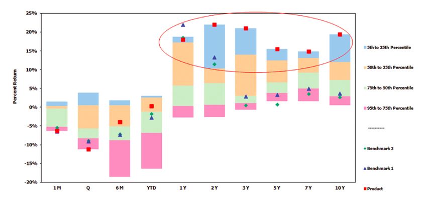
57Peer group analysis
58Peer groups a good benchmark?
Convenient - shows the edge, or lack thereof!
• Investable: NO
• Unambiguous: NO
• Measurable: YES
• Independent: NO
• Relevant: MAYBE
Issues: classification bias, survivorship bias, prone to snapshot
assessments – end point bias, can be gamed…
59End point bias
The same fund ranked in the top quartile when looking at
trailing periods
60Only one benchmark please!
Peer
Asset Class Cash/Hurdle Index
Group
Equities (EQ) ✔
Fixed Income (FI) ✔
Use as a secondary
tool to assess
Commodities (COM) ✔ performance
versus competition,
✔ ✔ and attribute
Real Estate (RE)
(RE PE/ REFs) (REITS) returns
Hedge Funds (HF) ✔
Private Equity (PE) ✔
61Basic Performance Comparison
Measures
62Time Weighted Return
• Cumulates returns over time
• Gives an equal weight to each result, regardless of the dollar
amount invested
• Returns are calculated daily and geometrically linked over
time
• Time-weighted methods do not consider the effect of
contributions or withdrawals on the portfolio
63Time Weighted Return
Investor 1 invests $1M on Dec 31. On Aug 15 of the following
year, his portfolio is valued at $1,162,484. At that point, he adds
$100,000, bringing total value to $1,262,484. By the end of the
year, portfolio has decreased in value to $1,192,328.
1st period return = ($1,162,484 - $1,000,000) / $1,000,000 =
16.25%
2nd period return = ($1,192,328 - ($1,162,484 + $100,000)) /
($1,162,484 + $100,000) = -5.56%
Time-weighted over the two time periods = (1 + 16.25%) x (1 + (-
5.56%)) - 1 = 9.79%
64How is my portfolio doing on an
absolute return basis?
• An absolute return measure allows direct alignment with
investment objective
• No comparison to a benchmark or peer
• Relevant for goal based investing agnostic of market or
benchmark performance
300 Portfolio Absolute Return Benchmark
250
Portfolio Ann. TWR=
200 6.45%
150
100
50
Jan-00 Jan-02 Jan-04 Jan-06 Jan-08 Jan-10 Jan-12 Jan-14 Jan-16
65How is my portfolio doing on a
relative return basis?
• Shows the portfolio is doing relative to SAA benchmark after
incorporating for drift and actively set tactical weights
300 Portfolio SAA
250 Portfolio Ann. TWR= 6.45%
SAA Ann. TWR = 5.70%
200
150
100
50
Jan-00 Jan-02 Jan-04 Jan-06 Jan-08 Jan-10 Jan-12 Jan-14 Jan-16
66Sharpe Ratio
• Measures portfolio excess return generated over the risk free
rate per unit of risk taken
• Implies that one is left with the premium that is independent
of total risk
• Provides easy comparison of portfolios and best used as a
ranking metric
Sharpe Ratio = (Ra - Rf) / σa
Ra is the portfolio return
Rf is the risk free rate
σa is the standard deviation of the portfolio return
67Sharpe Ratio
• Portfolio Sharpe = (6.45% - 0.60%) / 8.16% = 0.72
• SAA Sharpe = (5.70% - 0.60%) / 7.46% = 0.68
• Pitfalls
– It is a ranking criterion only
– Negative Sharpe is meaningless
– Does not incorporate higher moments
– Upward movement is penalized via higher volatility
– Doesn’t distinguish between active and passive return
– Not so useful when comparing strategies with vastly different trading
frequencies (e.g. HFT versus low frequency)
68Treynor Measure
• Measures outperformance over market or benchmark (beta)
• Independent of portfolio risk meaning one can compare two
portfolios even though they have different betas
Treynor Measure= (Ra - Rb) / βa
Ra is the portfolio return
Rb is the risk free rate
βa is the beta of the portfolio
69Treynor Measure
• Portfolio Treynor Measure = (6.45% - 0.60%) / 1.22 = 0.048
• Pitfalls
– Doesn’t quantify value added by active portfolio management
– It is a ranking criterion only
– Unlike Sharpe which applicable to all portfolios, Treynor uses relative
market risk or beta and hence is applicable only to well diversified
portfolios
70Jensen’s Alpha
• Measure of a security’s excess return with respect to the
expected return given by Capital Asset Pricing Model
Jensen’s Alpha = Ra - [Rb + βa*(Rm - Rb)]
= 6.45% - [0.60% + 1.22*(5.70% - 0.60%)]= -0.39%
Ra is the portfolio return
Rb is the risk free rate
Rm is the market return
βa is the beta of the portfolio
• Pitfalls: It only allows an absolute measurement of active
return
71Sharpe vs Treynor vs Jensen
Sharpe Treynor Jensen’s
Return Beta Std. Dev
Ratio Measure Alpha
Manager
10% 0.90 11% 0.91 0.11 0.03
A
Manager
14% 1.03 20% 0.70 0.14 0.06
B
Manager
15% 1.02 27% 0.56 0.15 0.07
C
Assuming risk free rate of 0% and benchmark return of 8%
Don’t forget: this is a snap shot, analyzing across time is crucial to assess
72
stability of these rankingsThe rebalancing decision
73Portfolio Setting
SAA Min Max Current
Allocation Allocation Allocation Allocation
Equity 25% 20% 30% 20.0%
Bonds 20% 15% 25% 12.6%
Commodities 5% 0% 10% 4.0%
Hedge Funds 15% 10% 20% 21.4%
Real Estate 10% 10% 20% 11.0%
Private Equity 25% 20% 30% 31.0%
Should we rebalance? - YES
74Can we rebalance effectively?
MOST PROBABLY NOT
• Low trading liquidity (potentially due to illiquid investments)
• Subscription/Redemption windows : time taken to
subscribe/redeem post request
• Lock-ins : investment can’t be redeemed at all
• Investment size: accurate rebalancing simply not possible
unless portfolio is of significant size
• High transaction costs and taxation
Factor in these considerations – set wider SAA bands
75Thank you.
76You can also read