Information Bottleneck for Estimating Treatment Effects with Systematically Missing Covariates - MDPI
←
→
Page content transcription
If your browser does not render page correctly, please read the page content below
entropy
Article
Information Bottleneck for Estimating Treatment
Effects with Systematically Missing Covariates
Sonali Parbhoo *,† , Mario Wieser , Aleksander Wieczorek             and Volker Roth
 Department of Mathematics and Computer Science, University of Basel, Basel CH 4051, Switzerland;
 mario.wieser@unibas.ch (M.W.); aleksander.wieczorek@unibas.ch (A.W.); volker.roth@unibas.ch (V.R.)
 * Correspondence: sparbhoo@seas.harvard.edu
 † Current address: John A. Paulson School of Engineering and Applied Sciences, Harvard University,
    Cambridge, MA 02138, USA.

 Received: 29 January 2020; Accepted: 27 March 2020; Published: 29 March 2020

 Abstract: Estimating the effects of an intervention from high-dimensional observational data is a
 challenging problem due to the existence of confounding. The task is often further complicated in
 healthcare applications where a set of observations may be entirely missing for certain patients at test
 time, thereby prohibiting accurate inference. In this paper, we address this issue using an approach
 based on the information bottleneck to reason about the effects of interventions. To this end, we first
 train an information bottleneck to perform a low-dimensional compression of covariates by explicitly
 considering the relevance of information for treatment effects. As a second step, we subsequently
 use the compressed covariates to perform a transfer of relevant information to cases where data are
 missing during testing. In doing so, we can reliably and accurately estimate treatment effects even
 in the absence of a full set of covariate information at test time. Our results on two causal inference
 benchmarks and a real application for treating sepsis show that our method achieves state-of-the-art
 performance, without compromising interpretability.

 Keywords: information bottleneck; mutual information; causal effect; average treatment effect;
 confounding; systematically missing; sufficient covariate; healthcare

1. Introduction
     Reasoning about the effects of an intervention is a key question across many applications such as
healthcare [1,2], finance [3] and public policy [4,5]. In general, making such predictions on the basis of
observational data containing only past actions, covariates and their outcomes is challenging, since
we do not have access to the precise mechanism that led to a particular action choice. Specifically, the
actions observed in the data may be determined by variables that also impact the outcome, resulting
in confounding that otherwise biases predictions if unaccounted for (e.g., socioeconomic status may
dictate what kinds of treatments a patient can afford and also affect their overall outcomes) [6].
Correcting for such confounding is thus crucial when estimating the effects of an intervention.
The problem is especially more challenging where a set of measurements is missing or systematically
missing for some patients at test time. Systematic missingness is a structured missingness where
a fixed set of variables is unavailable for a proportion of the data of interest, often as a result of
resource limitations at a particular time. It is a frequently occurring problem in many application areas:
For instance, a doctor treating patients with HIV may have access to both the genotype and phenotype
data for a particular study group of patients, but have a potentially larger group of patients outside
the study group, for whom genotype data are unavailable as a result of the medical costs associated
with genotyping. Here, estimating treatment effects for these patients requires integrating over all the
missing variables—an infeasible task in high-dimensional settings.

Entropy 2020, 22, 389; doi:10.3390/e22040389                                    www.mdpi.com/journal/entropy
Entropy 2020, 22, 389                                                                               2 of 18

     A naive strategy to address the problem of systematic missingness in the data is simply to remove
those features that are missing at test time, from the set of training data entirely and use a model
trained only on the reduced space of features to infer treatment effects. However, this approach
discards information that may be relevant in the training data for inferring outcomes. Alternatively,
one might use multiple imputation or other imputation-based techniques to first impute the incomplete
dimensions for the same purpose [7,8]. These methods work by generating a copy of the dataset in
which the missing values are computed on the basis of an imputation model. The procedure is repeated
several times in multiple imputation such that variations in the missing data can be accounted for.
Unfortunately in high-dimensional settings with systematic missingness, imputation-based solutions
can have large inaccuracies, particularly if many dimensions are missing. As a result, several other
approaches have been developed to account for data missingness during training by additionally
assuming for instance, hidden confounding. These methods typically try to build try to build a
joint model on the basis of noisy representatives or proxies of confounders (see for instance [9–12]).
However in high-dimensional-settings, it is unclear what these representatives might be or whether our
data meet such assumptions. Importantly, regardless of these assumptions none of these approaches
addresses systematic missingness at test time.
     A more natural approach would be to assume one could measure everything that is relevant
for estimating treatment effects for a subset of the patients, and attempt to transfer this distribution
of information to a potentially larger set of test patients. However, this is a challenging task given
the high dimensionality of the data that we must condition on in order to infer treatment effects. In
this paper, we address the problem from a decision-theoretic perspective of causal inference. Our
goal is to reliably estimate treatment effects where data are systematically missing at test time. To
do so, we work under the common assumption of strong ignorability. Our approach is based on the
Information Bottleneck (IB) method [13,14] that was originally introduced as a compression technique
to compress information about a random variable X while preserving relevant information about a
different random variable Y. Here, we use the IB to learn a sufficient reduction of the confounding
information for inferring treatment outcomes. A graphical overview of our approach is provided in
Figure 1.

Paper Contributions
      Our contributions may be summarised as follows:

•     First, we develop a method based on the Information Bottleneck to learn a compressed and
      interpretable representation of confounding.
•     Based on this representation, we learn equivalence classes among patients such that the causal
      effect for a specific patient can be approximated using the specific causal effect of the subgroups.
•     We subsequently transfer this information to a set of test cases where data is systematically
      missing at test time.
•     We demonstrate on two causal inference benchmark data sets and a real world application for
      treating sepsis that our approach outperforms existing approaches.

     The organisation of the remainder of the paper is as follows. Section 2 briefly reviews related
work, while Section 3 introduces our approach to inferring treatment outcomes using the Information
Bottleneck principle. In Section 4, we present our results on two popular causal inference benchmarks
and two real world applications. Section 5 concludes the work with final remarks, and outlines
directions for future research.
Entropy 2020, 22, 389                                                                                          3 of 18

                                                                     Clinical Data
                                Training Patients with                                   Test Patients with
                                                                     and Patient
                                Complete Information                                  Incomplete Information
                                                                       Histories

                                     Encoder                                                 Encoder
                                     Network             Genetic                             Network
                                                          Data

                                                              Knowledge Transfer

                                                         Compression of Confounding

                                                                    Decoder
                                                                    Network

                                                 Patient Outcomes             Treatment

      Figure 1. Graphical overview of our approach. We learn a discretised low-dimensional representation
      of confounding using the Information Bottleneck. As a result, we learn equivalence classes among the
      data such that we can use this information approximate the treatment effect for cases where data are
      systematically missing at test time.

2. Related Work
     A large amount of research in machine learning is targeted towards causal discovery with the aim
of learning the underlying causal graph from observational data (e.g., [15,16]). We instead focus on
causal deduction where the causal graph is known, and the task is rather to quantify the treatment effect
of one variable on another. In this vein, many existing works have been dedicated to counterfactual
reasoning and deep latent variable models. Since our key methodological contribution is based on a
deep-variant of the information bottleneck, we discuss these and other related models in this section.

2.1. Potential Outcomes and Counterfactual Reasoning
     Counterfactual reasoning (CR) has drawn large attention, particularly in the medical community.
Counterfactual models are essentially rooted in causal inference and may be used to determine the
causal effects of an intervention. These models are formalised in terms of potential outcomes [17–19].
Assume we have two choices of taking a treatment t, and not taking a treatment (control) c. Let
Yt denote the outcomes under t and Yc denote outcomes under the control c. The counterfactual
approach assumes that there is a pre-existing joint distribution P(Yt , Yc ) over outcomes. This joint
distribution is hidden since t and c cannot be applied simultaneously. Applying an action t thus only
reveals Yt , but not Yc . In this setting, computing the effect of an intervention involves computing the
difference between when an intervention is made and when no treatment is applied [20,21]. We would
subsequently choose to treat with t if,

                                                   E[ L(Yt )] ≤ E[ L(Yc )]                                        (1)

for loss L over Yt and Yc respectively. Potential outcomes are typically applied to cross-sectional
data [22,23] and sequential time settings. Notable examples of models for counterfactual reasoning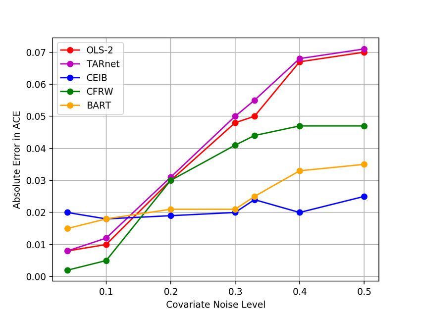
Entropy 2020, 22, 389                                                                                  4 of 18

include Johansson et al. [6] and Bottou et al. [24]. Specifically, Johansson et al. [6] propose a neural
network architecture called TARnet to estimate the effects of interventions. Similarly, Gaussian Process
CR (GPCR) models are proposed in Schulam and Saria [22,23] and further extended to the multitask
setting in Alaa and van der Schaar [2]. Off-policy evaluation methods in reinforcement learning (RL)
offer another perspective for reasoning about counterfactuals, and have been extensively explored to
estimate the outcomes of a particular policy or series of treatments based on retrospective observational
data (see for example Dudík et al. [25], Thomas and Brunskill [26], Jiang and Li [27]). Unlike each of
these techniques though, we focus specifically on estimating treatment effects where covariates are
systematically missing at test time.

2.2. Decision-Theoretic View of Causal Inference
     The decision theoretic approach to causal inference focuses on studying the effects of causes
rather than the causes of effects [28]. Here, the key question is what is the effect of the causal action
on the outcome? The outcome may be modelled as a random variable Y for which we can set up a
decision problem. That is, at each point, the value of Y is dependent on whether t or c is selected. The
decision-theoretic view of causal inference considers the distributions of outcomes given the treatment
or control, Pt and Pc and explicitly computes an expected loss of Y with respect to each action choice.
Finally, the choice to treat with t is made using Bayesian decision theory if,

                                       EY ∼ Pt [ L(Y )] ≤ EY ∼ Pc [ L(Y )].                               (2)

     Thus in this setting, causal inference involves comparing the expected losses over the hypothetical
distributions Pt and Pc for outcome Y. In this paper, we formulate our model in terms of the
decision-theoretic perspective of causal inference.

2.3. Estimating Treatment Effects with Missing Covariates
     A sizeable amount of work has previously been done on causal inference with missing data.
In particular, [29] propose using a latent mixture model to perform multiple imputation in order to
estimate treatment effects and compute propensity scores. Similarly, Cham and West [30] present
an empirical example of the performance of propensity score estimation methods when adapted
to missing covariates. More recently, Kallus et al. [31] performed a low-rank matrix factorisation
on a noisy set of covariate matrices to deduce a set of confounders based on which one can infer
treatment effects. The approach is general enough to adapt to scenarios where covariates are missing at
random and can be used as a preprocessing step for other bias correction techniques such as propensity
reweighting. Unlike these approaches, we make use of the IB criterion to adjust for the effects of
confounding and learn treatment effects. We specifically focus on a different type of missingness,
namely systematic missingness at test time.

2.4. The Information Bottleneck
     Let the Kullback Leibler divergence between two probability distributions p and q be denoted as
                                    p( X )
DKL ( p( X )||q( X )) = E p(X ) log q(X ) which is non-negative. Let I ( X; Z ) denote the mutual information
between X and Z where I ( X; Z ) = DKL ( p( X, Z )|| p( X ) p( Z ). Given two random variables X and Y, the
IB method [13] searches for a third random variable Z that, while compressing X, retains information
about Y. The resulting problem is defined as:

                                       min p(z| x) I ( X; Z ) − λI ( Z; Y ),                              (3)

where λ is a parameter that trades off the degree of compression of X with preservation of Y. The
classical IB method assumes that variables satisfy the Markov relation Z − X − Y, i.e., that given
X, Z and Y are conditionally independent. In its classical form, the IB principle is defined only for
Entropy 2020, 22, 389                                                                               5 of 18

discrete random variables. However, in recent years, multiple IB relaxations and extensions, such as
for Gaussian [32] and meta-Gaussian variables [33], have been proposed. Among these extensions, is
the latent variable (deep) formulation of the IB method that first appeared in [34], and then in [14,35].
Ref. [34] demonstrate how optimal representations of deep neural networks can be expressed in terms
of information dropout based on the IB method, while in parallel [14] consider variational lower
bounds on the information bottleneck problem for optimisation. The latter requires an analytically
solvable form of the lower bound in order to learn an optimal representation, while [34] propose
methods to learn this representation without such forms. Importantly, both [34] and [14] assume the
model adheres to the data generating process described by structural equations of the form,

                                             z = f ( x ) + ηz ,                                        (4)
                                             y = g ( z ) + ηy ,                                        (5)

where ηy , ηz are noise terms independent of Z and X respectively. These equations give rise to a
conditional independence relation that is different to the classical formulation, i.e., X − Z − Y where
given Z, X and Y are conditionally independent. While both independences from the classical IB and
latent variable formulation cannot hold in the same graph, Wieczorek and Roth [36] show that it is
possible to lift the original IB assumption in the context of the deep IB by optimising a lower bound on
the mutual information between Z and Y. In this paper, we use the latent variable formulation of the
IB and extend the formulation to deduce treatment effects where covariates are systematically missing
at test time.

2.5. Latent Variable Models
     Various probabilistic modelling techniques have been developed for similar tasks; for instance,
Ref. [37] build implicit causal models for application to genome-wide association studies. Similarly,
deep latent variable models have also received remarkable attention and been applied to a variety
of problems. Among these, variational autoencoders (VAEs) employ the reparameterisation trick
introduced in [38,39] to infer a variational approximation over the posterior distribution of the latent
space p(z| x ). Important work in this direction includes Kingma et al. [40] and Jang et al. [41]. Most
closely related to the work we present here, is the application of VAEs in a healthcare setting by
Louizos et al. [12]. Here, the authors introduce a Cause-Effect VAE (CEVAE) to estimate the causal
effect of an intervention in the presence of noisy proxies. It has been shown that there are several close
connections between the VAE framework and the latent variable formulation of the IB [14]. The latter
is essentially a VAE where X is replaced by Y in the decoder. Finally, Kaltenpoth and Vreeken [42]
propose using Probabilistic PCA to deduce a set of confounders and reason about treatment effects.
Unlike both of the aforementioned methods however, our approach considers a different causal graph
and specifically uses the IB method to learn a compressed representation of the covariate information
for reasoning about treatment effects where covariates are systematically missing at test time.

3. Method
      In recent years, there has been a growing interest in the connections between the IB principle
and deep neural networks [14,35,43]. In this section, we present a model using the IB principle, for
estimating the effects of an intervention in scenarios where covariates are systematically missing during
testing. Throughout the rest of this paper, we will refer to our approach as a Cause–Effect Information
Bottleneck (CEIB). Specifically, we combine the non-linear expressiveness of neural networks with the
IB criterion to learn a suitable representation of confounding, which we use to make inferences about
treatment effects. Our model thus consists of three main steps:

1.    First we perform a low-dimensional compression of covariate information using the Information
      Bottleneck to identify a discretised representation of confounding.
Entropy 2020, 22, 389 6 of 18
2. We use the representation to learn equivalence classes among patients, such that the treatment
effect for a specific patient can be approximated using the treatment effect of the equivalence
class associated with them.
3. Finally, we transfer this information to a set of test cases where data are systematically missing at
test time.
In what follows, we present our model and interpret our results from the decision-theoretic
perspective of causal inference [28]. We elaborate on each of above steps in the next sections. The
majority of the work we present here is based on Parbhoo [44].
3.1. Quantifying Causal Effects
Our goal in this paper is to make predictions about the causal effects of an intervention by
estimating the the Average Causal Effect (ACE) (or average treatment effect) [28] of an intervention T
on outcomes Y. In the interventional regime or setting, this is possible by actively intervening and
assigning treatments, or by performing an experimental study, e.g., randomised control trial to directly
measure the effects of introducing an intervention on subjects. Let FT = 0 and FT = 1 denote the
interventional setting where we actively assign or intervene on T. Here, the ACE is given by simply
measuring the difference in the outcomes of patients assigned to each intervention FT = 0 and FT = 1.
That is, the ACE is formally given by
ACE : = E[Y | FT = 1] − E[Y | FT = 0]. (6)
In general, however, it is not always possible to perform interventions to reason about treatment
effects directly, due to the costs and risks that may be incurred. As a result, we must frequently rely
on observational data to make inferences about treatment effects. The hallmark of learning from
observational data is that the actions observed in the data depend on variables which might also affect
the outcome, hence resulting in confounding. In the observational setting, the ACE can be written as:
ACE : = E[Y | T = 1, FT = ∅] − E[Y | T = 0, FT = ∅], (7)
where FT = ∅ denotes the fact that we no longer have control over the intervention/treatment
assignment and simply observe T as a random variable. Importantly, because of the influence of
confounding, the ACE in Equations (6) and (7) are in general, not equal unless we assume ignorable
treatment assignments or assume the conditional independence relation Y ⊥ ⊥ FT | T. This assumption
expresses that the distribution of Y | T is the same in the interventional and observational regimes,
and is equivalent to the setting where there is no confounding.
For the more general case where confounding is present, the treatment assignment FT may only
be ignored when estimating Y if provided a sufficient covariate, Z, and T [28]. Here, Z is a sufficient
covariate for the effect of T on outcome Y if Z ⊥
⊥ FT and Y ⊥ ⊥ FT | ( Z, T ). In this case, it can be shown
by Pearl’s backdoor criterion [20] that the ACE may be defined in terms of the Specific Causal Effect
(SCE),
ACE : = E[SCE( Z ) | FT = ∅] (8)
where
SCE( Z ) : = E[Y | Z, T = 1, FT = ∅] − E[Y | Z, T = 0, FT = ∅]. (9)
Overall, the SCE may be viewed as an equivalent of the ACE, restricted to a subspace of the
population with a certain value of Z = z. In this paper, we identify a low-dimensional representation
of confounding using the Information Bottleneck Principle. We discretise this representation such that
we can identify subgroups of the population with certain covariates. Importantly, the SCE enables usEntropy 2020, 22, 389 7 of 18
to approximate treatment effects for patients with systematically missing data at test time by assigning
them to similar subgroups of the population on the basis of their covariates.
3.2. Problem Formulation
Let X = ( X1 , X2 ) denote the set of patient covariates (confounders) based on which we would like
to estimate treatment effects. During training we assume that all covariates X ∈ Rd can be observed.
These correspond to, for instance, the measurements of a set of patients participating in a medical
study, where dimension d is large. Outside the study at test time however, we assume covariates X1 are
not observable, e.g., due to the expensive data acquisition process. This corresponds to having a fixed
set of features that are systematically missing for a subset of patients during testing. Let Y ∈ R denote
the outcomes following treatments T. For simplicity and ease of comparison with prior methods
on existing benchmarks, we consider treatments T that are binary, but our method is applicable for
any general T. We assume that all confounders are measurable (also known as strong ignorability)
during training and testing. That is, the set of confounders is measurable across all patients and do
not comprise the systematically missing covariates during testing. The causal graph corresponding to
our model is shown in Figure 2a. Finally, we assume that low-dimensional Z does not capture any
post-treatment variables, that may otherwise bias predictions. Under these assumptions, estimating
the ACE requires computing a distribution Y | Z, T, provided Z is a sufficient covariate. In what follows,
we use the IB to learn such a sufficient covariate that allows us to approximate the distribution Y | Z, T
in Figure 2a.
qη (v2 |x2 ) pθ (y|z, t)
Y X2 Y
V2
X Z Z
V1
FT T X1 T
qφ (v1 |x1 ) pψ (t|z)
(a)
(b)
Figure 2. (a) Influence diagram of the Cause-Effect Information Bottleneck (CEIB) . Red and green
circles correspond to observed and latent random variables respectively, while blue rectangles represent
interventions. We identify a low-dimensional representation Z of covariates X to estimate the effects
of an intervention on outcome Y where data are systematically missing at test time. (b) Graphical
illustration of the CEIB. Orange rectangles represent deep networks parameterising the random
variables. Our encoder networks qφ (v1 | x ) and qη (v2 | x ) try to minimise the first two terms in
Equation (10), while the decoder pθ (y|t, z) tries to minimise the last term in Equation (10).
3.3. IB Method for Performing a Sufficient Reduction of the Covariate
We now develop an extended formulation of the Information Bottleneck namely CEIB, for
estimating the effects of an intervention. Specifically, the new IB formulation enables us to learn
a low-dimensional, interpretable compression of the relevant information during training such that
we obtain a sufficiently reduced covariate Z. Based on this information, we can subsequently infer
treatment effects where covariates may be systematically missing at test time. To do so, we consider
the following adapted parametric form of the IB,
max − Iφ (V1 ; X1 ) − Iη (V2 ; X2 ) + λIφ,θ,ψ,η ( Z; (Y, T )), (10)
φ,θ,ψ,η
where V1 and V2 are compressed discrete representations of the covariates, Z = (V1 , V2 ) is a
concatenation of V1 and V2 and I represents the mutual information parameterised by φ, ψ, θ, and η
respectively. We assume a parametric form of the conditionals qφ (v1 | x ), qη (v2 | x ), pθ (y|t, z), pψ (t|z).Entropy 2020, 22, 389 8 of 18
The modified IB criterion in Equation (10) reflects that we would like to obtain an optimal compression
Z of X while simultaneously retaining information about Y (given T). The first two terms of our new
IB formulation are given by:
Iφ (V1 ; X1 ) = DKL (qφ (v1 | x1 ) p( x1 )|| p(v1 ) p( x1 )) = E p( x1 ) DKL (qφ (v1 | x1 )|| p(v1 )) (11)
Iη (V2 ; X2 ) = DKL (qη (v2 | x2 ) p( x2 )|| p(v2 ) p( x2 )) = E p( x2 ) DKL (qη (v2 | x2 )|| p(v2 )), (12)
while the last term has the form:
Iφ,θ,ψ,η ( Z; (Y, T )) ≥ E p( x,y,t) E pφ,η (z| x) log pθ (y|t, z) + log pψ (t|z) + H (y, t)1 ,
(13)
where H (y, t) = −E p(y,t) log p(y, t) is the entropy of (y, t). The lower bound follows from the
fact that the mutual information between Z and Y, T can be expressed as a sum of the expected
value of log pθ (y|t, z) + log pψ (t|z), entropy H (y, t) and two KL-divergences, which are by definition
non-negative [36]. Specifically, in Equation (13) we bound I ( Z; Y ) using the result from [36] such that
we no longer require the original IB conditional independence assumption described in Section 2.4.
Importantly, optimising the criterion in Equation (10) enables us to learn a sufficiently reduced covariate
Z which can be used to accurately estimate the ACE using Equation (8). Unlike other approaches for
inferring treatment effects, the Lagrange parameter λ in the IB formulation in Equation (10) allows us
to adjust the degree of compression, which, in this context, enables us to learn a sufficient statistic Z. In
particular, adjusting λ enables us to explore a range of such representations from having a completely
insufficient covariate where Y ⊥ 6 ⊥ FT | ( Z, T ), to a completely sufficient compression of confounding
where Y ⊥ ⊥ FT | ( Z, T ) — a property crucial for auditing and interpreting the resulting predictions.
Note that in general, we are free to choose a suitable parametric form in order to optimise Equation (10).
In what follows, we describe how to do so with neural networks.
3.4. Implementation of the IB Method
We now describe how to implement and optimise the criterion in Equation (10). The proposed
architecture of our model is illustrated in Figure 2b. I ( X; V1) and I ( X; V2) are parameterised by two
neural networks (also known as encoder networks). The encoder networks try to minimise the first
two terms in Equation (10). I ( Z; (Y, T )) is parameterised by another neural network (known as the
decoder network). The decoder network tries to minimise the last term of the loss in Equation (10).
For our encoder architectures, we specifically compress X to obtain discrete latent representations
V1 and V2 of the covariate information. To do so, we make use of the Gumbel softmax
reparameterisation trick [41] to draw samples Z from a categorical distribution with probabilities π.
Here,
z = one_hot(arg max[ gi + log πi ]), (14)
i
where one_hot refers to a one-hot feature encoding and g1 , g2 , . . . , gk are samples drawn from
Gumbel(0,1). The softmax function is used to approximate the arg max in Equation (14), and generate
k-dimensional sample vectors w ∈ ∆k−1 , where
exp((log(πi ) + gi )/τ )
wi = k
,i = 1, . . . , k. (15)
∑ j=1 exp((log(π j ) + g j )/τ )
and τ is the softmax temperature parameter.Entropy 2020, 22, 389 9 of 18
For our decoder network, we use an architecture similar to the TARnet [6], where we replace
conditioning on high-dimensional covariates X with conditioning on reduced covariate Z. We can
thus formulate the conditionals as,
pψ (t|z) = Bern(σ( f 1 (z)))
pθ (y|t, z) = N (µ = µ̂, ς2 = ŝ), (16)
with logistic function σ (·), and outcome Y given by a Gaussian distribution parameterised with a
TARnet with µ̂ = t f 2 (z) + (1 − t) f 3 (z). Note that the terms f k correspond to neural networks. While
distribution p(t|z) is included to ensure the joint distribution over treatments, outcomes and covariates
is identifiable, in practice, our goal is to approximate the effects of a given T on Y. Hence, we train our
model in a teacher forcing fashion by using the true treatment assignments T from the data and fixing
the Ts at test time.
Overall, by using the Gumbel softmax reparameterisation trick to obtain a discrete representation
of relevant information, we can learn equivalence classes among patients based on which we can
compute the SCE for each group using sufficient covariate Z via Equation (9). This has an important
implication. Specifically, it means that during training our method reduces covariates X to a sufficiently
compressed covariate Z. If a subset X1 of X is unavailable after training, we can still use the learnt Z
to compute the ACE during testing, since the m-graphs associated with Figure 2a no longer contain
only random variables and hence become degenerate. Thus at test time, we can subsequently assign
an example with missing covariates to its relevant equivalence class. Here, computing the SCE allows
us potentially to tailor treatments to specific groups based on Z rather than an entire population– an
important aspect in healthcare where patients are typically heterogeneous. Based on the SCE, we can
also compute the population-level effects of an intervention via the ACE from Equation (8). In the
absence of the latent compression via CEIB and the discrete representation of relevant information, it
would not be possible to transfer knowledge from examples with complete information to cases with
systematically missing information, since estimating treatment effects would require integrating over
all the covariates—an infeasible task in high dimensions.
4. Experiments
The lack of ground truth in real world data makes evaluating causal inference methods a difficult
problem. To overcome this issue, existing approaches typically consider using semi-synthetic data sets
where outcomes and treatment assignments are fully known, or randomised control trial experiments.
Our goal is to demonstrate the ability of CEIB to accurately infer treatment effects, while simultaneously
learning a low-dimensional, interpretable representation of confounding in cases where covariate
information is systematically missing at test time. For this purpose, we consider a task-based on a
randomised control experiment and a second semi-synthetic task for treating low birth-weight twins.
Additionally, we demonstrate the performance of our approach on a real high-dimensional task for
managing and treating sepsis. In our experiments, we report both the SCE and ACE values for this
purpose.
4.1. Infant Health and Development Program
The Infant Health and Development Program (IHDP) [45,46] is a randomised control experiment
assessing the impact of educational intervention on the outcomes of pre-mature low birth-weight
infants born between 1984 and 1985. Measurements from children and their mothers were collected
for studying the effects of childcare and home visits from a trained specialist on test scores. The study
contains information about the children and their mothers/caregivers. Data on children includes
sex, birth weight, head circumference and other health indices. Information about mothers includes
maternal age and race, as well as educational achievement. Together, these data comprise our data
set, denoted as X. Treatments or interventions T are binary indicators corresponding to participationEntropy 2020, 22, 389 10 of 18
in the IHDP child development centres, while outcomes Y correspond to the IQ-test score measured
following intervention.
Like Hill [46], features and treatment assignments are extracted from the real world clinical
trial, and selection bias is introduced in the data by artificially removing a non-random portion of
the treatment group, in particular children with non-white mothers. In total, the resulting data set
then consists of 747 subjects (139 treated, 608 control), each represented by 26 covariates measuring
the properties of the child and their mother. We subsequently divide this data set into 60/10/30%
training/validation/test sets. For our setup, we use encoder and decoder architectures with 3 hidden
layers and train the model using Adam as an optimiser with a learning rate of 0.001. We train our model
with four 3-dimensional Gaussian mixture components, although our method can be applied, without
loss of generality, to any number of dimensions. We compare the performance of CEIB for predicting
the ACE against several existing baselines, first for the case where no covariates are systematically
missing at test time, and subsequently by considering the best performing baselines for the case
where covariates are systematically missing during testing. Specifically, we consider the following
baselines: OLS-1 is a least squares regression; OLS-2 uses two separate least squares regressions to fit
the treatment and control groups respectively; TARnet is a feedforward neural network from Shalit
et al. [47]; KNN is a k-nearest neighbours regression; RF is a random forest; BNN is a balancing neural
network [6]; BLR is a balancing linear regression [6]; BART is a Bayesian Additive Regression Tree
model [48,49]; CFRW is a counterfactual regression that uses the Wasserstein distance [47].
Table 1. (a) Within-sample and out-of sample error in estimating the true Average Causal Effect (ACE)
across models on the complete data set. A smaller value indicates better performance. Bold values
indicate the method with the best performance. (b) Out-of-sample error in estimating the ACE across
models using a reduced set of 22 covariates at test time. CEIB outperforms all the baselines in both (a)
and (b).
(a)
−s out −o f −s
Method ewithin
ACE e ACE
OLS-1 0.73 ± 0.04 0.94 ± 0.06
OLS-2 0.14 ± 0.01 0.34 ± 0.02
KNN 0.14 ± 0.01 0.79 ± 0.05
BLR 0.72 ± 0.04 0.93 ± 0.05
TARnet 0.26 ± 0.01 0.28 ± 0.01
BNN 0.37 ± 0.03 0.42 ± 0.03
RF 0.73 ± 0.05 0.96 ± 0.06
BART 0.23 ± 0.01 0.33 ± 0.02
CEVAE 0.34 ± 0.01 0.46 ± 0.02
CFRW 0.25 ± 0.01 0.27 ± 0.01
CEIB 0.11 ± 0.01 0.21 ± 0.01
(b)
out −o f −s
Method e ACE
TARnet .34 ± 0.01
CFRW 0.49 ± 0.02
BART 0.39 ± 0.02
CEIB 0.23 ± 0.01
Experiment 1: In the first experiment, we compared the performance of CEIB for estimating the
ACE against the baselines when using the complete set of measurements at test time. In Table 1(a) we
report the difference between the true ACE and our CEIB estimate since we have de-randomised the
data. We repeat this on multiple data splits. Evidently, CEIB outperforms existing approaches. To
demonstrate that we can transfer the relevant information to cases where covariates are systematicallyEntropy 2020, 22, 389 11 of 18
missing at test time, we artificially excluded n = 3 covariates that have a moderate correlation
with ethnicity at test time. We compute the ACE and compare this to the performance of the three
best performing baselines namely, TARnet, CFRW and BART applied to the reduced set of covariates
(Table 1(b)). If we extend this to the extreme case of removing 8 covariates at test time, the out-of-sample
error in predicting the ACE increases to 0.29 +/− 0.02. Thus CEIB achieves the highest predictive
performance for both in-sample and out-of-sample predictions, even with systematically missing
covariates. Overall, these results largely match our expectations since prediction accuracy for all
the approaches decreases when covariates are systematically missing at test time. We attribute
the difference in performance to the way in which CEIB uses covariate information when making
predictions. Unlike any of the other methods, CEIB specifically extracts only the information that is
relevant for making predictions, and uses this to learn a suitable representation of confounding to infer
treatment effects.
Experiment 2: Building on Experiment 1, we perform an analysis of the latent space of our model
to assess whether we learn a sufficiently reduced covariate. We use the IHDP data set as before, but
this time consider both the data before introducing selection bias (analogous to a randomised study),
as well as after introducing selection bias by removing a non-random proportion of the treatment group
as before (akin to a de-randomised study). We plot the information curves illustrating the number of
latent dimensions required to reconstruct the output for the terms I ( Z; (Y, T )) and I ( Z, T ) respectively
for varying values of λ. These results are shown in Figure 3a,b. Theoretically, we should be able to
examine the shape of the curves to identify whether a sufficiently reduced covariate has been obtained.
In particular, when a study is randomised, the sufficient covariate Z should have no impact on the
treatment T. In this case, the mutual information I ( Z, T ) should be approximately zero and the curve
should remain flat for varying values of I ( Z, X ). This result is confirmed in Figure 3a. The information
curves in Figure 3b additionally demonstrate our model’s ability to account for confounding when
predicting the overall outcomes: when data are de-randomised, we are able to reconstruct treatment
outcomes more accurately. Specifically, the point at which each of the information curves saturates
is the point at which we have learnt a sufficiently reduced covariate based on which we can infer
treatment effects. Overall, the results from Figure 3a,b highlight another benefit of using CEIB for
estimating treatment outcomes: in particular, by adjusting the Lagrange parameter λ, CEIB allows for
a task-dependent adjustment of the latent space. This adjustment allows one to explore a full range of
solutions across the information curve, from having a completely insufficient covariate to a completely
sufficient compression of the covariates where the information curve saturates. In the absence of the IB
objective, this is not possible. Overall, we are able to learn a low-dimensional representation that is
consistent with the ethnicity confounder. By conditioning on this representation, we can thus account
for its effects when predicting treatment outcomes.
We also analysed the discretised latent space by comparing the proportions of ethnic groups of
test subjects in each cluster in the de-randomised setting. These results are shown in Figure 4 where
we plot a hard assignment of test subjects to clusters on the basis of their ethnicity. Evidently, the
clusters exhibit a clear structure with respect to ethnicity. In particular, Cluster 2 in Figure 4b has a
significantly higher proportion of non-white members in the de-randomised setting. The discretisation
also allows us to calculate the SCE for each cluster. In general, Cluster 2 tends to have a lower SCE
than the other groups. This is consistent with how the data were de-randomised, since we removed a
proportion of the treated instances with non-white mothers. Conditioning on this kind of information
is thus crucial to be able to accurately assess the impact of educational intervention on test scores.
Finally, we assess the error in estimating the ACE when varying the number of mixture components in
Figure 5. When the number of clusters is larger, the clusters get smaller and it becomes more difficult
to reliably estimate the ACE since we average over the cluster members to account for partial covariate
information at test time. Here, model selection is made by observing where the error in estimating the
ACE stabilises (anywhere between 4 and 7 mixture components).Entropy 2020, 22, 389 12 of 18
5 5 5 7
0.7 4 5 5
4 4 5
3 6
3 3 4
0.6 3
5
3
0.5 3
4
I(Z; (Y, T))
I(Z; T)
2 4 4 5 5 5
0.4 2 3
5 3 3
5 3
3 3 3 4 4 5
0.3
2 2
2 2
0.2 2 1 2
De-randomised De-randomised
Randomised Randomised
0.1 0
2.1 3.6 5.3 6.9 8.1 11.4 13 14.5 16 17.4 2.1 3.6 5.3 6.9 8.1 11.4 13 14.5 16 17.4
I(Z; X) I(Z; X)
(a) (b)
Figure 3. (a) Information curves for I ( Z; T ) and (b) I ( Z; (Y, T )) with de-randomised and randomised
data respectively. When the data are randomised, the value of I ( Z; T ) is close to zero. The differences
between the curves illustrates confounding. When data are de-randomised, we are able to estimate
treatment effects more accurately by accounting for this confounding.
60 60 50
50 80 50 40
Proportion in Cluster (%)
Proportion in Cluster (%)
Proportion in Cluster (%)
Proportion in Cluster (%)
40 40
60 30
30 30
40 20
20 20
20 10
10 10
0 0 0 0
African-American White African-American White African-American White African-American White
Ethnicity Ethnicity Ethnicity Ethnicity
(a) SCE: 4.9 (b) SCE: 2.7 (c) SCE: 4.3 (d) SCE: 4.1
Figure 4. Illustration of the proportion of major ethnic groups within the four clusters. Grey and orange
indicate de-randomised and randomised data respectively. For better visualisation, we only report the
two main clusters which include the majority of all patients. The first cluster in (a) is a neutral cluster.
The second cluster in (b) shows an enrichment of information in the African-American group. Clusters
3 and 4 in (c) and (d) respectively, show an enrichment of information in the White group. Overall, the
clusters exhibit a distinct structure with respect to the known ethnicity confounder. Moreover, each of
the clusters is associated with different Specific Causal Effect (SCE) values. In particular, the second
cluster has a lower SCE which suggests that educational intervention for these members has less of an
impact on outcomes—a result consistent with our de-randomisation strategy.
.
1.2
1.0
Out-of-sample error in ACE
0.8
0.6
0.4
0.2
2 4 6 8 10
Number of clusters
Figure 5. Out-of-sample error in ACE with a varying number of clusters.Entropy 2020, 22, 389 13 of 18
4.2. Binary Treatment Outcome on Twins
As a second application, we make use of data about twin births in the USA between 1989 and
1991 [50]. Here, treatment T = 1 is a binary indicator of being the heavier twin at birth, while outcome
Y corresponds to the mortality within a year after birth. Since mortality is rare, we consider only same
sex twins with weights less than 2 kg, which results in 11,984 pairs of twins. Each twin has a set of
46 covariates comprising our dataset X. These covariates include information about parents of the
twins such as their level of education, race, incidence of renal disease, diabetes, smoking etc., as well as
whether the birth took place in hospital or at home and the number of gestation weeks prior to birth.
To simulate an observational study, we selectively hide one of the twins. Treatments T are allocated
based on a single variable which is highly correlated with the outcome: GESTAT10, the number of
gestation weeks prior to birth. This has values from 0 to 9 that correspond to the weeks of gestation
before birth, i.e., birth before 20 weeks gestation, 20-27 weeks of gestation, etc. Analogous to [12], we
set treatment to t| x, z ∼ Bern(σ(wo> x + wh (z/10 − 0.1))) for wo ∼ N (0, 0.1I ), wh ∼ N (5, 0.1), where z
is GESTAT10 and x are the 45 remaining covariates. We compared the performance of CEIB to TARnet,
OLS 2, BART, CFRW in terms of the errors in estimating the ACE. These results are summarised in
Figure 6.
Figure 6. Absolute error in ACE estimation for Twins task. CEIB outperforms baselines over varying
levels of covariate noise.
Overall, CEIB outperforms each of the baselines under varying levels of covariate noise. We
attribute this to the fact that CEIB extracts only the information that is relevant for making predictions
(via the IB criterion) in order to draw inferences about the effects of interventions.
4.3. Sepsis Management
We also illustrate the performance CEIB on the real-world task of managing and treating sepsis.
Sepsis is one of the leading causes of mortality within hospitals and treating septic patients is highly
challenging, since outcomes vary with interventions and there are no universal treatment guidelines.
For this experiment, we make use of data from the Multiparameter Intelligent Monitoring in Intensive
Care (MIMIC-III) database [51]. We focus specifically on patients satisfying Sepsis-3 criteria (16
804 patients in total). For each patient, we have a 48-dimensional set of physiological parameters
including demographics, lab values, vital signs and input/output events, where certain covariates are
systematically missing. We denote this set as X. Our outcomes Y correspond to the odds of mortality,
while we binarise medical interventions T according to whether or not a vasopressor is administered.Entropy 2020, 22, 389 14 of 18
The data set is divided into 60%/20%/20% into training/validation/testing sets. We train our model
with six 4-dimensional Gaussian mixture components and analysed the information curves and cluster
compositions respectively.
The information curves for I ( Z; T ) and I ( Z; (Y, T )) are shown in Figure 7a and 7b respectively.
We observe that we can perform a sufficient reduction of the high-dimensional covariate information
to between four and six dimensions while achieving high predictive accuracy of outcomes Y. Since
there is no ground truth available for the sepsis task, we do not have access to the true confounding
variables. However, we can perform an analysis on the basis of the clusters obtained over the latent
space. Here, we see that we can characterise the patients in each cluster according to their initial
SOFA (Sequential Organ Failure Assessment) scores. SOFA scores range between 1 and 4 and are used
to track a patient’s stay in hospital. In Figure 8, we observe clear differences in cluster composition
relative to the SOFA scores. Clusters 2, 5 and 6 tend to have higher proportions of patients with lower
SOFA scores, while Clusters 3 and 4 have larger proportions of patients with higher SOFA scores.
This result suggests that a patient’s initial SOFA score is potentially a confounder when determining
how to administer subsequent treatments and predicting their odds of in-hospital mortality. This is
consistent with medical studies such as Medam et al. [52], Studnek et al. [53] where authors indicate
that high initial SOFA scores were likely to impact on their overall chances of survival and treatments
administered in hospital.
While we cannot quantify an error in estimating the ACE since we do not have access to the
counterfactual outcomes, we can still compute the ACE for the sepsis management task. Here,
we specifically observe a negative ACE value. This means that in general, treating patients with
vasopressors reduces the chances of mortality in comparison to not treating patients with vasopressors.
Overall, performing such analyses for tasks like sepsis may shed light on what information is relevant
for making predictions and reasoning about the effects of medical intervention. In turn, this may assist
in establishing potential therapy guidelines for better decision-making.
6 6
0.8 5 6
5
0.7
4 4
0.6
0.5
I(Z; T)
3 4
0.4
0.3
2
0.2
0.1
1.8 2.3 2.9 4.5 4.8 5.3 5.8 6.3 6.8 7.2
I(Z; X)
(a) (b)
Figure 7. Subfigures (a) and (b) illustrate the information curve I ( Z; T ) and I ( Z; (Y, T )) for the task of
managing sepsis. We perform a sufficient reduction of the covariates to 6-dimensions and are able to
approximate the ACE on the basis of this.Entropy 2020, 22, 389 15 of 18
35
50 40
30
Proportion in Cluster (%)
Proportion in Cluster (%)
Proportion in Cluster (%)
25 40
30
20 30
15 20
20
10
10
5 10
0 0 0
1 2 3 4 1 2 3 4 1 2 3 4
Initial SOFA Score Initial SOFA Score Initial SOFA Score
(a) SCE: -1.2 (b) SCE: -2.7 (c) SCE: 1.4
50
35 60
40 30 50
Proportion in Cluster (%)
Proportion in Cluster (%)
Proportion in Cluster (%)
25 40
30
20
30
20 15
20
10
10
5 10
0 0 0
1 2 3 4 1 2 3 4 1 2 3 4
Initial SOFA Score Initial SOFA Score Initial SOFA Score
(d) SCE: 2.1 (e) SCE: -3.8 (f) SCE: 1.7
Figure 8. Proportion of initial Sequential Organ Failure Assessment (SOFA) scores in each cluster. The
variation in initial SOFA scores across clusters suggests that it is a potential confounder of odds of
mortality when managing and treating sepsis.
5. Discussion
5.1. Low-Dimensional, Interpretable Representations of Confounding
Because CEIB is explicitly constrained to extract only the information that is relevant for making
predictions about outcomes, it is capable of learning a low-dimensional representation of confounding,
using which we can base our predictions. Specifically, by introducing a discrete clustering structure
in the latent space of our model, we can easily inspect and interpret the confounding effects. For the
IHDP experiment, this means we can learn a low-dimensional representation of the known ethnicity
confounder and account for its effects when predicting treatment outcomes. Earlier methods such as
Louizos et al. [12] use higher dimensional representations (in the order of 20 dimensions) to account
for these effects yet make less accurate predictions. A possible explanation for this is that the true
confounding effect is misrepresented. Consequently, modelling the task using the IB model alleviates
this issue. Similarly for the task of treating septic patients in ICU, we identified a low-dimensional latent
space of 6 dimensions for predicting the odds of mortality, where clusters exhibited a distinct structure
with respect to a patient’s initial SOFA score. Importantly, across all tasks, the low-dimensional
representation allows us to accurately identify confounders whilst retaining model interpretability.
5.2. Accurate Estimation of the Causal Effect with Systematically Missing Covariates during Testing
Unlike earlier approaches, CEIB can deal with systematically missing data during test time
through the introduction of a discretised latent space via the Gumbel softmax reparameterisation
trick. Based on this representation, we can learn equivalence classes among patients such that the
approximate the effects of treatments can be computed.
5.3. State-of-the-Art ACE Predictions That Are Robust against Confounding
Across the IHDP dataset, we see that predictions of the ACE are considerably more accurate than
existing approaches. In the IHDP case, we see reductions in the error in estimating the ACE up to
0.58 for in-sample predictions. This performance is sustained when making out-of-sample predictionsEntropy 2020, 22, 389 16 of 18
we see error reductions of between 0.04 and 0.73 in comparison with existing methods. Overall, we
attribute this increase in performance directly to the fact that CEIB extracts only the information that is
relevant for making predictions. Proxy-based approaches such as Louizos et al. [12] do not explicitly
trade off learning meaningful representations of confounders and achieving accurate predictions.
In contrast, we can explicitly inspect the information curves in Figure 3b and adjust compression
parameter λ to expose a relevant representation of confounding. If we set λ = 13 in accordance to
Figure 3b, we require only a 4-dimensional representation to adequately account for and uncover the
true confounding effect Z (as shown in Figure 4b). This produces more accurate predictions as a result.
6. Conclusions
We have presented a novel approach to estimate causal relationships with systematically missing
covariates at test time. This is an important problem particularly in healthcare, since doctors frequently
have access to certain routine measurements, but may have difficulty acquiring others such as genotype
information. For this purpose, we analysed the role of a sufficient covariate in the context of the IB
framework. This included introducing a discrete latent space to facilitate transferring knowledge
to cases where information was systematically missing—a task that is otherwise infeasible in high
dimensions. In doing so, we could estimate the causal effect if parts of the covariates are missing
during test time, while accounting for confounding. In contrast to previous methods, the compression
parameter λ in the IB framework allows for a task-dependent adjustment of the latent dimensionality.
Our extensive experiments showed that our method outperforms state-of-the-art approaches on
multiple synthetic and real world datasets. More broadly, since handling systematic missingness is a
highly relevant problem in healthcare, we view this as step towards improving these systems on a
larger scale. Directions for future work include adapting our approach to infer other causal concepts
such as the Effect of Treatment on Treated (ETT) for instance, through the use of instrumental variables;
as well as relating the model to existing double robustness techniques and propensity scoring methods.
Author Contributions: Conceptualisation, S.P.; Writing, S.P., M.W., A.W.; Supervision, V.R. All authors have read
and agree to the published version of the manuscript.
Funding: Sonali Parbhoo is supported by the Swiss National Science Foundation project P2BSP2 184359 and
NIH1R56MH115187. Mario Wieser is partially supported by the NCCR MARVEL and grant 51MRP0158328
(SystemsX.ch) funded by the Swiss National Science Foundation.
Conflicts of Interest: The authors declare no conflict of interest.
References
1. Wager, S.; Athey, S. Estimation and inference of heterogeneous treatment effects using random forests. J. Am.
Stat. Assoc. 2017, 113, 1228–1242 [CrossRef]
2. Alaa, A.M.; van der Schaar, M. Bayesian Inference of Individualized Treatment Effects using Multi-task
Gaussian Processes. In Proceedings of the 31st Conference on Neural Information Processing Systems
(NIPS 2017), Long Beach, CA, USA, 4–9 December 2017.
3. Imbens, G.W.; Wooldridge, J.M. Recent developments in the econometrics of program evaluation. J. Econ.
Lit. 2009, 47, 5–86. [CrossRef]
4. Athey, S.; Imbens, G.W. The state of applied econometrics: Causality and policy evaluation. J. Econ. Perspect.
2017, 31, 3–32. [CrossRef]
5. Dehejia, R.H.; Wahba, S. Causal effects in nonexperimental studies: Reevaluating the evaluation of training
programs. J. Am. Stat. Assoc. 1999, 94, 1053–1062. [CrossRef]
6. Johansson, F.D.; Shalit, U.; Sontag, D. Learning Representations for Counterfactual Inference. In Proceedings
of the 33rd International Conference on Machine Learning: New York, NY, USA, 19–24 June 2016;
pp. 3020–3029.
7. Little, R.J.; Rubin, D.B. Statistical Analysis with Missing Data; John Wiley & Sons: Chichester, UK, 2019;
Volume 793.
8. Rubin, D.B. Inference and missing data. Biometrika 1976, 63, 581–592. [CrossRef]Entropy 2020, 22, 389 17 of 18
9. Greenland, S.; Lash, T. Bias Analysis. In Modern Epidemiology; Lippincott Williams & Wilkins: Philadelphia,
PA, USA, 2008; pp. 345–380.
10. Pearl, J. On measurement bias in causal inference. arXiv 2012, arXiv:1203.3504.
11. Kuroki, M.; Pearl, J. Measurement bias and effect restoration in causal inference. Biometrika 2014, 101, 423–437.
[CrossRef]
12. Louizos, C.; Shalit, U.; Mooij, J.M.; Sontag, D.; Zemel, R.; Welling, M. Causal Effect Inference with Deep
Latent-Variable Models. In Proceedings of the Advances in Neural Information Processing Systems 30,
Long Beach, CA, USA, 4–9 December 2017; pp. 6446–6456.
13. Tishby, N.; Pereira, F.C.; Bialek, W. The information bottleneck method. arXiv 2000, arXiv:physics/0004057.
14. Alemi, A.A.; Fischer, I.; Dillon, J.V.; Murphy, K. Deep Variational Information Bottleneck. arXiv 2016,
arXiv:1612.00410.
15. Mooij, J.M.; Peters, J.; Janzing, D.; Zscheischler, J.; Schölkopf, B. Distinguishing cause from effect using
observational data: methods and benchmarks. J. Mach. Learn. Res. 2016, 17, 1103–1204.
16. Peters, J.; Mooij, J.M.; Janzing, D.; Schölkopf, B. Causal discovery with continuous additive noise models.
J. Mach. Learn. Res. 2014, 15, 2009–2053.
17. Splawa-Neyman, J. Sur les applications de la théorie des probabilités aux experiences agricoles: Essai des
principes. Roczniki Nauk Rolniczych 1923, 10, 1–51. (In Polish)
18. Splawa-Neyman, J. On the Application of Probability Theory to Agricultural Experiments. Essay on
Principles. Section 9. Stat. Sci. 1990, 5, 465–472. [CrossRef]
19. Rubin, D.B. Bayesian inference for causal effects: The role of randomization. Ann. Stat. 1978, 6, 34–58.
[CrossRef]
20. Pearl, J. Causality; Cambridge University Press: Cambridge, UK, 2009.
21. Morgan, S.L.; Winship, C. Counterfactuals and Causal Inference; Cambridge University Press: Cambridge,
UK, 2015.
22. Schulam, P.; Saria, S. Reliable Decision Support using Counterfactual Models. In Proceedings of the Advances
in Neural Information Processing Systems 30, Long Beach, CA, USA, 4–9 December 2017; pp. 1697–1708.
23. Schulam, P.; Saria, S. What-If Reasoning using Counterfactual Gaussian Processes. In Proceedings of
the Advances in Neural Information Processing Systems 30: Annual Conference on Neural Information
Processing Systems 2017, Long Beach, CA, USA, 4–9 December 2017; pp. 1696–1706.
24. Bottou, L.; Peters, J.; Quiñonero-Candela, J.; Charles, D.X.; Chickering, D.M.; Portugaly, E.; Ray, D.; Simard,
P.; Snelson, E. Counterfactual reasoning and learning systems: The example of computational advertising.
J. Mach. Learn. Res. 2013, 14, 3207–3260.
25. Dudík, M.; Langford, J.; Li, L. Doubly robust policy evaluation and learning. arXiv 2011, arXiv:1103.4601.
26. Thomas, P.; Brunskill, E. Data-efficient off-policy policy evaluation for reinforcement learning. In
Proceedings of the 33rd International Conference on Machine Learning: New York, NY, USA, 19–24 June
2016; pp. 2139–2148.
27. Jiang, N.; Li, L. Doubly Robust Off-policy Value Evaluation for Reinforcement Learning. arXiv 2016,
arXiv:1511.03722.
28. Dawid, P. Fundamentals of Statistical Causality; Technical report; Department of Statistical Science; University
College London: London, UK, 2007.
29. Mitra, R.; Reiter, J.P. Estimating propensity scores with missing covariate data using general location mixture
models. Stat. Med. 2011, 30, 627–641. [CrossRef]
30. Cham, H.; West, S.G. Propensity score analysis with missing data. Psychol. Methods 2016, 21, 427. [CrossRef]
31. Kallus, N.; Mao, X.; Udell, M. Causal inference with noisy and missing covariates via matrix factorization.
In Proceedings of the Advances in Neural Information Processing Systems 31 (NIPS 2018): Montréal, QC,
Canada, 3–8 December 2018; pp. 6921–6932.
32. Chechik, G.; Globerson, A.; Tishby, N.; Weiss, Y. Information bottleneck for Gaussian variables. J. Mach.
Learn. Res. 2005, 6, 165–188.
33. Rey, M.; Roth, V. Meta-Gaussian Information Bottleneck. In Proceedings of the Advances in Neural
Information Processing Systems 25 (NIPS 2012): Lake Tahoe, NV, USA, 3–6 December 2012; pp. 1925–1933.
34. Achille, A.; Soatto, S. Information dropout: Learning optimal representations through noisy computation.
IEEE Trans. Pattern Anal. Mach. Intell. 2018, 40, 2897–2905. [CrossRef] [PubMed]You can also read