Intriguing properties of neural networks
←
→
Page content transcription
If your browser does not render page correctly, please read the page content below

Intriguing properties of neural networks

    Christian Szegedy         Wojciech Zaremba           Ilya Sutskever            Joan Bruna
       Google Inc.           New York University           Google Inc.         New York University

         Dumitru Erhan                   Ian Goodfellow                       Rob Fergus
           Google Inc.               University of Montreal              New York University
                                                                             Facebook Inc.

                                              Abstract

         Deep neural networks are highly expressive models that have recently achieved
         state of the art performance on speech and visual recognition tasks. While their
         expressiveness is the reason they succeed, it also causes them to learn uninter-
         pretable solutions that could have counter-intuitive properties. In this paper we
         report two such properties.
         First, we find that there is no distinction between individual high level units and
         random linear combinations of high level units, according to various methods of
         unit analysis. It suggests that it is the space, rather than the individual units, that
         contains of the semantic information in the high layers of neural networks.
         Second, we find that deep neural networks learn input-output mappings that are
         fairly discontinuous to a significant extend. Specifically, we find that we can cause
         the network to misclassify an image by applying a certain imperceptible pertur-
         bation, which is found by maximizing the network’s prediction error. In addition,
         the specific nature of these perturbations is not a random artifact of learning: the
         same perturbation can cause a different network, that was trained on a different
         subset of the dataset, to misclassify the same input.

1   Introduction

Deep neural networks are powerful learning models that achieve excellent performance on visual and
speech recognition problems [9, 8]. Neural networks achieve high performance because they can
express arbitrary computation that consists of a modest number of massively parallel nonlinear steps.
But as the resulting computation is automatically discovered by backpropagation via supervised
learning, it can be difficult to interpret and can have counter-intuitive properties. In this paper, we
discuss two counter-intuitive properties of deep neural networks.
The first property is concerned with the semantic meaning of individual units. Previous works
[6, 13, 7] analyzed the semantic meaning of various units by finding the set of inputs that maximally
activate a given unit. The inspection of individual units makes the implicit assumption that the units
of the last feature layer form a distinguished basis which is particularly useful for extracting seman-
tic information. Instead, we show in section 3 that random projections of (x) are semantically
indistinguishable from the coordinates of (x). Moreover, this puts into question the conjecture that
neural networks disentangle variation factors across coordinates. Generally, it seems that it is the
entire space of activations, rather than the individual units, that contains the bulk of the semantic
information. A similar, but even stronger conclusion was reached recently by Mikolov et al. [12]
for word representations, where the various directions in the vector space representing the words are
shown to give rise to a surprisingly rich semantic encoding of relations and analogies. At the same

                                                   1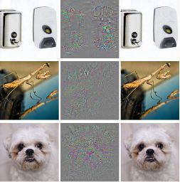
time, the vector representations are well-defined up to a rotation of the space, so the individual units
of the vector representations are unlikely to contain semantic information.
The second property is concerned with the stability of neural networks with respect to small per-
turbations to their inputs. Consider a state-of-the-art deep neural network that generalizes well on
an object recognition task. We expect such network to be robust to small perturbations of its in-
put, because small perturbation cannot change the object category of an image. However, we find
that applying an imperceptible non-random perturbation to a test image, it is possible to arbitrarily
change the network’s prediction (see figure 5). These perturbations are found by optimizing the
input to maximize the prediction error. We term the so perturbed examples “adversarial examples”.
It is natural to expect that the precise configuration of the minimal necessary perturbations is a
random artifact of the normal variability that arises in different runs of backpropagation learning.
Yet, we found that adversarial examples are relatively robust, and are shared by neural networks
with varied number of layers, activations or trained on different subsets of the training data. That is,
if we use one neural to generate a set of adversarial examples, we find that these examples are still
statistically hard for another neural network even when it was trained with different hyperparemeters
or, most surprisingly, when it was trained on a different set of examples.
These results suggest that the deep neural networks that are learned by backpropagation have nonin-
tuitive characteristics and intrinsic blind spots, whose structure is connected to the data distribution
in a non-obvious way.

2   Framework
Notation We denote by x 2 Rm an input image, and (x) activations values of some layer. We first
examine properties of the image of (x), and then we search for its blind spots.
We perform a number of experiments on a few different networks and three datasets :
       • For the MNIST dataset, we used the following architectures [11]
           – A simple fully connected, single layer network with a softmax classifier on top of it.
              We refer to this network as “softmax”.
           – A simple fully connected network with two hidden layers and a classifier. We refer to
              this network as “FC”.
           – A classifier trained on top of autoencoder. We refer to this network as “AE”.
           – A standard convolutional network that achieves good performance on this dataset:
              it has one convolution layer, followed by max pooling layer, fully connected layer,
              dropout layer, and final softmax classifier. Referred to as “Conv”.
       • The ImageNet dataset [3].
           – Krizhevsky et. al architecture [9]. We refer to it as “AlexNet”.
       • ⇠ 10M image samples from Youtube (see [10])
           – Unsupervised trained network with ⇠ 1 billion learnable parameters. We refer to it as
              “QuocNet”.
For the MNIST experiments, we use regularization with a weight decay of . Moreover, in some
experiments we split the MNIST training dataset into two disjoint datasets P1 , and P2 , each with
30000 training cases.

3   Units of: (x)
Traditional computer vision systems rely on feature extraction: often a single feature is easily inter-
pretable, e.g. a histogram of colors, or quantized local derivatives. This allows one to inspect the
individual coordinates of the feature space, and link them back to meaningful variations in the input
domain. Similar reasoning was used in previous work that attempted to analyze neural networks that
were applied to computer vision problems. These works interpret an activation of a hidden unit as a
meaningful feature. They look for input images which maximize the activation value of this single
feature [6, 13, 7, 4].

                                                   2
(a) Unit sensitive to lower round stroke. (b) Unit sensitive to upper round stroke, or
lower straight stroke.
(c) Unit senstive to left, upper round (d) Unit senstive to diagonal straight
stroke. stroke.
Figure 1: An MNIST experiment. The figure shows Images that maximize the activation of various units
(maximum stimulation in the natural basis direction). Images within each row share semantic properties.
(a) Direction sensitive to upper straight (b) Direction sensitive to lower left loop.
stroke, or lower round stroke.
(c) Direction senstive to round top stroke. (d) Direction sensitive to right, upper
round stroke.
Figure 2: An MNIST experiment. The figure shows images that maximize the activations in a random direction
(maximum stimulation in a random basis). Images within each row share [remove many] semantic properties.
The aforementioned technique can be formally stated as visual inspection of images x0 , which satisfy
(or are close to maximum attainable value):
x0 = arg max h (x), ei i
x2image set
However, our experiments show that any random direction v 2 Rn gives rise to similarly inter-
pretable semantic properties. More formally, that maximize the activations in a random direction
are also semantically related.
x0 = arg max h (x), vi
x2image set
This suggest that the natural basis is not better than a random basis in for inspecting the properties
of (x). Moreover, it puts into question the notion that neural networks disentangle variation factors
across coordinates.
First, we evaluated the above claim using a convolutional neural network trained on MNIST. For the
”image set” we used test set. Figure 1 shows images that maximize the activations in the natural
basis, and Figure 2 shows images that maximize the activation in random directions. In both cases
the resulting images share many high-level similarities.
Next, we repeated our experiment on an AlexNet, where we used the validation set for the ”image
set”. Figures 3 and 4 compare the natural basis to the random basis on the trained network. The
rows appear to be semantically meaningful for both the single unit and the combination of units.
Although such analysis gives insight on the capacity of to generate invariance on a particular
subset of the input distribution, it does not explain the behavior on the rest of its domain. We shall
see in the next section that has counterintuitive properties in the neighbourhood of almost every
point form data distribution.
4 Blind Spots in Neural Networks
So far, unit-level inspection methods had relatively little utility beyond confirming certain intuitions
regarding the complexity of the representations learned by a deep neural network [6, 13, 7, 4].
Global, network level inspection methods can be useful in the context of explaining classification
3(a) Unit sensitive to white flowers. (b) Unit sensitive to postures.
(c) Unit senstive to round, spiky flowers. (d) Unit senstive to round green or yellow
objects.
Figure 3: Experiment performed on ImageNet. Images stimulating single unit most (maximum stimulation in
natural basis direction). Images within each row share many semantic properties.
(a) Direction sensitive to white, spread (b) Direction sensitive to white dogs.
flowers.
(c) Direction sensitive to spread shapes. (d) Direction sensitive to dogs with brown
heads.
Figure 4: Experiment performed on ImageNet. Images giving rise to maximum activations in a random direc-
tion (maximum stimulation in a random basis). Images within each row share many semantic properties.
decisions made by a model [1] and can be used to, for instance, identify the parts of the input which
led to a correct classification of a given visual input instance (in other words, one can use a trained
model for weakly-supervised localization). Such global analyses are useful in that they can make us
understand better the input-to-output mapping represented by the trained network.
Generally speaking, the output layer unit of a neural network is a highly nonlinear function of its
input. When it is trained with the cross-entropy loss (using the softmax activation function), it
represents a conditional distribution of the label given the input (and the training set presented so
far). It has been argued [2] that the deep stack of non-linear layers in between the input and the
output unit of a neural network are a way for the model to encode a non-local generalization prior
over the input space. In other words, it is possible for the output unit to assign non-significant
(and, presumably, non-epsilon) probabilities to regions of the input space that contain no training
examples in their vicinity. Such regions can represent, for instance, the same objects from different
viewpoints, which are relatively far (in pixel space), but which share nonetheless both the label and
the statistical structure of the original inputs.
It is implicit in such arguments that local generalization—in the very proximity of the training
examples—works as expected. And that in particular, for a small enough radius " in the vicinity of
a given training input x, an x" which satisfies ||x x" || < " will get assigned a high probability
of the correct class by the model. This kind of smoothness prior is typically valid for computer
vision problems, where imperceptibly tiny perturbations of a given image do not normally change
the underlying class.
Our main result is that for deep neural networks, the smoothness assumption that underlies many
kernel methods does not hold. Specifically, we show that by using a simple optimization procedure,
we are able to find adversarial examples, which are obtained by imperceptibly small perturbations
to a correctly classified input image, so that it is no longer classified correctly. This can never occur
with smooth classifiers by their definition.
In some sense, what we describe is a way to traverse the manifold represented by the network in an
efficient way (by optimization) and finding adversarial examples in the input space. The adversarial
4(a) (b)
Figure 5: Adversarial examples generated for AlexNet [9].(Left) is correctly predicted sample, (center) dif-
ference between correct image, and image predicted incorrectly magnified by 10x (values shifted by 128 and
clamped), (right) adversarial example. Average distortion based on 64 examples is 0.006508.
examples represent low-probability (high-dimensional) “pockets” in the manifold, which are hard to
efficiently find by simply randomly sampling the input around a given example. Already, a variety
of recent state of the art computer vision models employ input deformations during training for
increasing the robustness and convergence speed of the models [9, 13]. These deformations are,
however, statistically inefficient, for a given example: they are highly correlated and are drawn from
the same distribution throughout the entire training of the model. We propose a scheme to make this
process adaptive in a way that exploits the model and its deficiencies in modeling the local space
around the training data.
We make the connection with hard-negative mining explicitly, as it is close in spirit: hard-negative
mining, in computer vision, consists of identifying training set examples (or portions thereof) which
are given low probabilities by the model, but which should be high probability instead, cf. [5]. The
training set distribution is then changed to emphasize such hard negatives and a further round of
model training is performed. As shall be described, the optimization problem proposed in this work
can also be used in a constructive way, similar to the hard-negative mining principle.
4.1 Formal description
We denote by f : Rm ! {1 . . . k} a classifier mapping image pixel value vectors to a discrete
label set. We also assume that f has an associated continuous loss function denoted by lossf :
Rm ⇥ {1 . . . k} ! R+ . For a given x 2 Rm image and target label l 2 {1 . . . k}, we aim to solve
the following box-constrained optimization problem:
• Minimize krk2 subject to:
1. f (x + r) = l
2. x + r 2 [0, 1]m
The minimizer r might not be unique, but we denote one such x + r for an arbitrarily chosen
minimizer by D(x, l). Informally, x + r is the closest image to x classified as l by f . Obviously,
D(x, f (x)) = f (x), so this task is non-trivial only if f (x) 6= l. In general, the exact computation
of D(x, l) is a hard problem, so we approximate it by using a box-constrained L-BFGS. Concretely,
we find an approximation of D(x, l) by performing line-search to find the minimum c > 0 for which
the minimizer r of the following problem satisfies f (x + r) = l.
• Minimize c|r| + lossf (x + r, l) subject to x + r 2 [0, 1]m
4.2 Experimental results
Our “minimimum distortion” function D has the following intriguing properties, which we will
demonstrate with qualitative and quantitative experiments in this section:
5(a) (b)
Figure 6: Adversarial examples for QuocNet [10]. A binary car classifier was trained on top of the last layer
features without fine-tuning. The examples on the left are recognized correctly as cars, while the images in the
middle are not recognized. The rightmost column is the magnified absolute value of the difference between the
two images.
1. For all the networks we studied (MNIST, QuocNet [10], AlexNet [9]), for each sample, we
always manage to generate very close, visually indistinguishable, adversarial examples that
are misclassified by the original network (see figure 5 for examples).
2. Cross model generalization: a relatively large fraction of examples will be misclassified by
networks trained from scratch with different hyper-parameters (number of layers, regular-
ization or initial weights).
3. Cross training-set generalization a relatively large fraction of examples will be misclassi-
fied by networks trained from scratch trained on a disjoint training set.
The above observations suggest that adversarial examples are somewhat universal and not just the
results of overfitting to a particular model or to the specific selection of the training set. They
also suggest that back-feeding adversarial examples to training might improve generalization of the
resulting models. Our preliminary experiments have yielded positive evidence on MNIST to support
this hypothesis as well: We have successfully trained a two layer 100-100-10 non-convolutional
neural network with a test error below 1.2% by keeping a pool of adversarial examples a random
subset of which is continuously replaced by newly generated adversarial examples and which is
mixed into the original training set all the time. For comparison, a network of this size gets to
1.6% errors when regularized by weight decay alone and can be improved to around 1.3% by using
carefully applied dropout. A subtle, but essential detail is that adversarial examples are generated
for each layer output and are used to train all the layers above. Adversarial examples for the higher
layers seem to be more useful than those on the input or lower layers.
For space considerations, we just present results for a representative subset (see table 1) of the
MNIST experiments we perfomed. The results presented here are consistent with those on a larger
variety of non-convolutional models. For MNIST, we do not have results for convolutional mod-
els yet, but our first qualitative experiments with AlexNet gives us reason to believe that convolu-
tional networks may behave similarly as well. Each of our models were trained with L-BFGS until
convergence. The first three models are linear classifiers that work on the pixel level with various
weight decay parameters
P 2 . All our examples use quadratic weight decay on the connection weights:
lossdecay = wi /k added to the total loss, where k is the number of units in the layer. One of
the models is trained with extremely high = 1 in order to test whether it is still possible to gen-
erate adversarial examples in this extreme setting as well. Two other models are a simple sigmoidal
neural network with two hidden layers and a classifier. The last model consists of a single layer
sparse autoencoder with sigmoid activations and 400 nodes with a softmax classifier. This network
has been trained until it got very high quality first layer filters and this layer was not fine-tuned. The
last column measures the minimum average pixelqlevel distortion necessary to reach 0% accuracy
P 0
(xi xi )2
on the training set. The distortion is measure by n between the original x and distorted
x0 images, where n = 784 is the number of image pixels. The pixel intensities are scaled to be in
the range [0, 1].
In our first experiment, we generate a set of adversarial instances for a given network and feed
these examples for each other network to measure the ratio of misclassified instances. The last
column shows the average minimum distortion that was necessary to reach 0% accuracy on the
whole training set. The experimental results are presented in table 2. The columns of the table show
the error (ratio of disclassified instances) on the so distorted training sets. The last two rows are
special and show the error induced when distorting by Gaussian noise. Note that even the noise
6(a) Even columns: adver- (b) Even columns: adver- (c) Randomly distorted
sarial examples for a linear sarial examples for a 200- samples by Gaussian noise
(softmax) classifier (std- 200-10 sigmoid network with stddev=1. Accuracy:
dev=0.06) (stddev=0.063) 51%.
Figure 7: Adversarial examples for MNIST compared with randomly distorted examples. Odd columns display
the original images. The adversarial examples generated for the specific model have accuracy 0% for the
respective model. Note that while the randomly distorted examples are hardly readable, still they are classified
correctly in half of the cases, while the adversarial examples are never classified correctly. Odd columns
correspond to original images, and even columns correspond to distorted counterparts.
Model Name Description Training error Test error Av. min. distortion
softmax1 Softmax with = 10 4 6.7% 7.4% 0.062
softmax2 Softmax with = 10 2 10% 9.4% 0.1
softmax3 Softmax with =1 21.2% 20% 0.14
N100-100-10 Sigmoid network = 10 5 , 10 5 , 10 6 0% 1.64% 0.058
N200-200-10 Sigmoid network = 10 5 , 10 5 , 10 6 0% 1.54% 0.065
AE400-10 Autoencoder with softmax = 10 6 0.57% 1.9% 0.086
Table 1: Tests of the generalization of adversarial instances on MNIST
softmax1 softmax2 softmax3 N100-100-10 N200-200-10 AE400-10 Av. distortion
softmax with = 10 4 100% 11.7% 22.7% 2% 3.9% 2.7% 0.062
softmax with = 10 2 87.1% 100% 35.2% 35.9% 27.3% 9.8% 0.1
softmax with =1 71.9% 76.2% 100% 48.1% 47% 34.4% 0.14
N100-100-10 28.9% 13.7% 21.1% 100% 6.6% 2% 0.058
N200-200-10 38.2% 14% 23.8% 20.3% 100% 2.7% 0.065
AE400-10 23.4% 16% 24.8% 9.4% 6.6% 100% 0.086
Gaussian noise, stddev=0.1 5.0% 10.1% 18.3% 0% 0% 0.8% 0.1
Gaussian noise, stddev=0.3 15.6% 11.3% 22.7% 5% 4.3% 3.1% 0.3
Table 2: Cross-model generalization of adversarial examples. The columns of the tables show the error induced
by distorted examples fed to the given model. The last column shows average distortion wrt. original training
set.
Model Error on P1 Error on P2 Error on Test Min Av. Distortion
M1 : 100-100-10 trained on P1 0% 2.4% 2% 0.062
M10 : 123-456-10 trained on P1 0% 2.5% 2.1% 0.059
M2 : 100-100-10 trained on P2 2.3% 0% 2.1% 0.058
Table 3: Models trained to study cross-training-set generalization of the generated adversarial examples. Errors
presented in table correpond to original not-distorted data, to provide a baseline.
with stddev 0.1 is greater than the stddev of our adversarial noise for all but one of the models.
Figure 7 shows a visualization of the generated adversarial instances for two of the networks used
in this experiment The general conclusion is that adversarial examples tend to stay hard even for
models trained with different hyperparameters. Although the autoencoder based version seems most
resilient to adversarial examples, it is not fully immune either.
Still, this experiment leaves open the question of dependence over the training set. Does the hardness
of the generated examples rely solely on the particular choice of our training set as a sample or does
this effect generalize even to models trained on completely different training sets?
To study cross-training-set generalization, we have partitioned the 60000 MNIST training images
into two parts P1 and P2 of size 30000 each and trained three non-convolutional networks with
7M1 M10 M2
Distorted for M1 (av. stddev=0.062) 100% 26.2% 5.9%
Distorted for M10 (av. stddev=0.059) 6.25% 100% 5.1%
Distorted for M2 (av. stddev=0.058) 8.2% 8.2% 100%
Gaussian noise with stddev=0.06 2.2% 2.6% 2.4%
Distorted for M1 amplified to stddev=0.1 100% 98% 43%
Distorted for M10 amplified to stddev=0.1 96% 100% 22%
Distorted for M2 amplified to stddev=0.1 27% 50% 100%
Gaussian noise with stddev=0.1 2.6% 2.8% 2.7%
Table 4: Cross-training-set generalization error rate for the set of adversarial examples generated for different
models. The error induced by a random distortion to the same examples is displayed in the last row.
sigmoid activations on them: Two, M1 and M10 , on P1 and M2 and P2 . The reason we trained two
networks for P1 is to study the cumulative effect of changing the hypermarameters and the training
sets at the same time. Models M1 and M2 share the same hyperparameters: both of them are 100-
100-10 networks, while M10 is a 123-456-10 network. In this experiment, we were distorting the
elements of the test set rather than the training set. Table 3 summarizes the basic facts about these
models. After we generate adversarial examples with 100% error rates with minimum distortion for
the test set, we feed these examples to the each of the models. The error for each model is displayed
in the corresponding column of the upper part of table 4. In the last experiment, we magnify the
0
effect of our distortion by using the examples x + 0.1 kxx0 xk x
2
rather than x0 . This magnifies the
distortion on average by 40%, from stddev 0.06 to 0.1. The so distorted examples are fed back
to each of the models and the error rates are displayed in the lower part of table 4. The intriguing
conclusion is that the adversarial examples remain hard for models trained even on a disjoint training
set, although their effectiveness decreases considerably.
4.3 Spectral Analysis of Instability
The previous section showed that the networks resulting from supervised learning are unstable with
respect to a particular family of perturbations. The instability is expressed mathematically as a
collection of pairs (xi , ni )i such that kni k but k (xi ; W ) (xi + ni ; W )k M > 0 for a
small value of , and for generic values of trainable parameters W . This suggests that the class of
unstable perturbations ni depends on the architecture of , but does not depend upon the particular
training parameters W .
The instability of (x; W ) can be partly explained by inspecting the upper Lipschitz constant of
each layer, defined as Lk > 0 such that
8 x, x0 , k k (x) 0
k (x )k Lk kx x0 k .
The rectified layers (both convolutional or fully connected) are defined by the mapping k (x) =
max(0, Wk x + bk ). Let (W ) and + (W ) denote respectively the lower and upper frame bounds
of W (i.e., its lowest and largest singular values). Since max(0, x) is contractive, it results that
Lk kWk k = + (Wk ). It results that a first measure of the instability of the network can be
obtained by simply computing the frame bounds of each of the linear operators. The max-pooling
layers are contractive, which implies that they do not increase the upper bounds, although they can
decrease the lower bounds. This effect is not considered in the present work.
If W denotes a generic 4-tensor convolutional layer with stride ,
( C )
X
Wx = xc ? wc,f [n1 , n2 ] ; f = 1 . . . , F ,
c=1
where xc denotes the c input feature image, then one can verify that its operator norm is given by
kW k = sup kA(!)k ,
!
where A(!) is the matrix whose rows are
1
8 f = 1 . . . F , A(!)f = wdc,f (! + l⇡ ) ; c = 1 . . . C , l = (0 . . . 1)2 .
Table 5 shows the upper and lower bounds computed from the ImageNet deep convolutional network
of [9]. It shows that instabilities can appear as soon as in the first convolutional layer.
8Layer Size Lower bound Upper bound
Conv. 1 3 ⇥ 11 ⇥ 11 ⇥ 96 0.1 20
Conv. 2 96 ⇥ 5 ⇥ 5 ⇥ 256 0.06 10
Conv. 3 256 ⇥ 3 ⇥ 3 ⇥ 384 0.01 7
Conv. 4 384 ⇥ 3 ⇥ 3 ⇥ 384 5 · 10 5 7.3
Conv. 5 384 ⇥ 3 ⇥ 3 ⇥ 256 0.03 11
FC. 1 9216 ⇥ 4096 0.09 3.12
FC. 2 4096 ⇥ 4096 10 4 4
FC. 3 4096 ⇥ 1000 0.25 4
Table 5: Frame Bounds of each convolutional layer
5 Discussion
We demonstrated that deep neural networks have counter-intuitive properties both with respect to
the semantic meaning of individual units and with respect to their discontinuities. The existence of
the adversarial negatives appears to be in contradiction with the network’s ability to achieve high
generalization performance. Indeed, if the network can generalize well, how can it be confused by
these adversarial negatives, which are indistinguishable from the regular examples? The explanation
is that the set of adversarial negatives is of extremely low probability, and thus is never (or rarely)
observed in the test set, yet it is dense (much like the rational numbers, and so it is found near every
virtually every test case.
References
[1] David Baehrens, Timon Schroeter, Stefan Harmeling, Motoaki Kawanabe, Katja Hansen, and Klaus-
Robert Müller. How to explain individual classification decisions. The Journal of Machine Learning
Research, 99:1803–1831, 2010.
[2] Yoshua Bengio. Learning deep architectures for ai. Foundations and trends® in Machine Learning,
2(1):1–127, 2009.
[3] Jia Deng, Wei Dong, Richard Socher, Li-Jia Li, Kai Li, and Li Fei-Fei. Imagenet: A large-scale hierarchi-
cal image database. In Computer Vision and Pattern Recognition, 2009. CVPR 2009. IEEE Conference
on, pages 248–255. IEEE, 2009.
[4] Dumitru Erhan, Yoshua Bengio, Aaron Courville, and Pascal Vincent. Visualizing higher-layer features
of a deep network. Technical Report 1341, University of Montreal, June 2009. Also presented at the
ICML 2009 Workshop on Learning Feature Hierarchies, Montréal, Canada.
[5] Pedro Felzenszwalb, David McAllester, and Deva Ramanan. A discriminatively trained, multiscale, de-
formable part model. In Computer Vision and Pattern Recognition, 2008. CVPR 2008. IEEE Conference
on, pages 1–8. IEEE, 2008.
[6] Ross Girshick, Jeff Donahue, Trevor Darrell, and Jitendra Malik. Rich feature hierarchies for accurate
object detection and semantic segmentation. arXiv preprint arXiv:1311.2524, 2013.
[7] Ian Goodfellow, Quoc Le, Andrew Saxe, Honglak Lee, and Andrew Y Ng. Measuring invariances in deep
networks. Advances in neural information processing systems, 22:646–654, 2009.
[8] Geoffrey E. Hinton, Li Deng, Dong Yu, George E. Dahl, Abdel rahman Mohamed, Navdeep Jaitly, An-
drew Senior, Vincent Vanhoucke, Patrick Nguyen, Tara N. Sainath, and Brian Kingsbury. Deep neural
networks for acoustic modeling in speech recognition: The shared views of four research groups. IEEE
Signal Process. Mag., 29(6):82–97, 2012.
[9] Alex Krizhevsky, Ilya Sutskever, and Geoff Hinton. Imagenet classification with deep convolutional
neural networks. In Advances in Neural Information Processing Systems 25, pages 1106–1114, 2012.
[10] Quoc V Le, Marc’Aurelio Ranzato, Rajat Monga, Matthieu Devin, Kai Chen, Greg S Corrado, Jeff Dean,
and Andrew Y Ng. Building high-level features using large scale unsupervised learning. arXiv preprint
arXiv:1112.6209, 2011.
[11] Yann LeCun and Corinna Cortes. The mnist database of handwritten digits, 1998.
[12] Tomas Mikolov, Kai Chen, Greg Corrado, and Jeffrey Dean. Efficient estimation of word representations
in vector space. arXiv preprint arXiv:1301.3781, 2013.
[13] Matthew D Zeiler and Rob Fergus. Visualizing and understanding convolutional neural networks. arXiv
preprint arXiv:1311.2901, 2013.
9You can also read