Introduction to Forecast Verification - Tressa L. Fowler, Tara L .Jensen, Barbara G. Brown
←
→
Page content transcription
If your browser does not render page correctly, please read the page content below

Introduction to Forecast
      Verification
Tressa L. Fowler, Tara L .Jensen, Barbara G.
                   Brown

   National Center for Atmospheric Research
            Boulder Colorado USA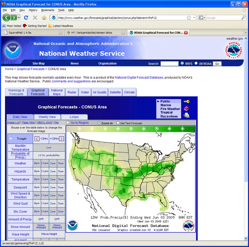
Outline
• Basic verification concepts                            • Categorical verification
   –   What is verification?                               statistics
   –   Why verify?                                             –   Contingency tables
   –   Identifying verification goals                          –   Thresholds
   –   Forecast “goodness”                                     –   Skill scores
   –   Designing a verification study                          –   Receiver Operating
   –   Types of forecasts and                                      Characteristic (ROC) curves
       observations
   –   Matching forecasts and                            • Continuous verification
       observations                                        statistics
   –   Verification attributes                                 –   Joint and Marginal distributions
   –   Miscellaneous issues                                    –   Scatter plots
   –   Questions to ponder: Who?                               –   Discrimination plots
       What? When? Where? Which?                               –   Conditional statistics and plots
       Why?
                                                               –   Commonly used verification
                                                                   statistics

         Copyright 2012, University Corporation for Atmospheric Research,
         all rights reserved
                                                                              2
What is verification?

      • Verification is the process of comparing forecasts
        to relevant observations
             – Verification is one aspect of measuring forecast goodness

      • Verification measures the quality of forecasts (as
        opposed to their value)

      • For many purposes a more appropriate term is
        “evaluation”

Copyright 2012, University Corporation for Atmospheric Research, all rights
                                                                              3
reserved
Why verify?
                     • Purposes of verification (traditional definition)

                            – Administrative purpose
                                  • Monitoring performance
                                  • Choice of model or model configuration
                                    (has the model improved?)

                            – Scientific purpose
                                  • Identifying and correcting model flaws
                                  • Forecast improvement

                            – Economic purpose
                                  • Improved decision making
                                  • “Feeding” decision models or decision support systems
Copyright 2012, University Corporation for Atmospheric Research, all rights
                                                                                            4
reserved
Identifying verification goals
What questions do we want to answer?
• Examples:
ü In what locations does the model have the best
performance?
ü Are there regimes in which the forecasts are better
or worse?
ü Is the probability forecast well calibrated (i.e.,
reliable)?
ü Do the forecasts correctly capture the natural
variability of the weather?
Other examples?
Copyright 2012, University Corporation for Atmospheric Research, all rights
5
reserved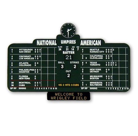
Identifying verification goals (cont.)
      • What forecast performance attribute should be
        measured?
             • Related to the question as well as the type of forecast
               and observation

      • Choices of verification statistics, measures,
        graphics
             • Should match the type of forecast and the attribute
               of interest
             • Should measure the quantity of interest (i.e., the
               quantity represented in the question)

Copyright 2012, University Corporation for Atmospheric Research, all rights
                                                                              6
reserved
Forecast “goodness”
      • Depends on the quality of the forecast

                           AND

      • The user and his/her application of the
        forecast information

Copyright 2012, University Corporation for Atmospheric Research, all rights
                                                                              7
reserved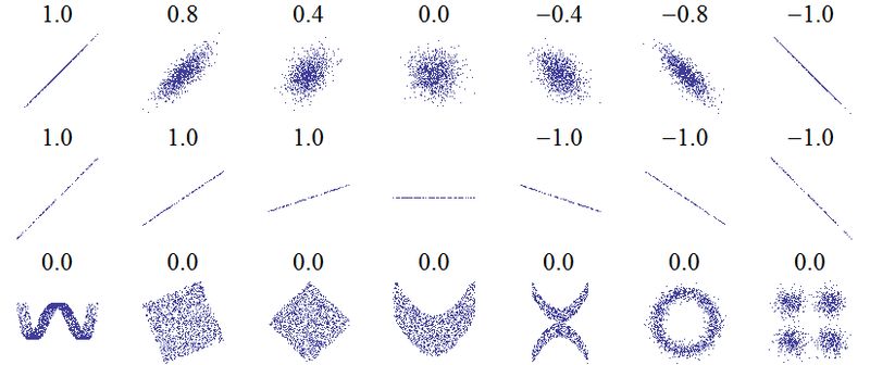
Good forecast or bad forecast?

                                             F                 O

Copyright 2012, University Corporation for Atmospheric Research,
                                                                   8
all rights reserved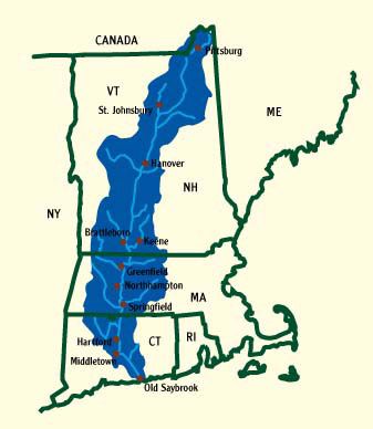
Good forecast or Bad forecast?

    If I’m a water
   manager for this                          F                 O
   watershed, it’s a
      pretty bad
      forecast…

Copyright 2012, University Corporation for Atmospheric Research,
                                                                   9
all rights reserved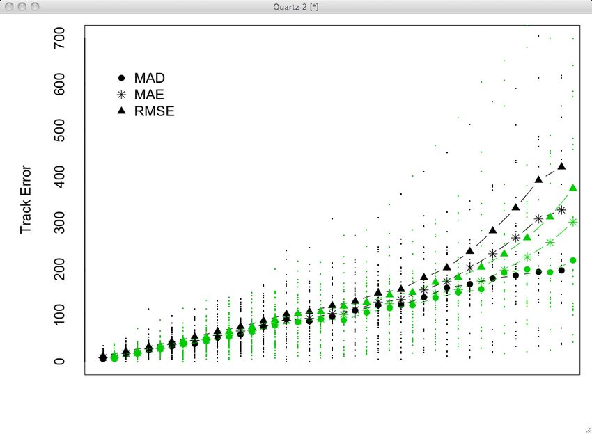
Good forecast or Bad forecast?

                        F         O
A                      Flight Route                         B

                                 O

                 If I’m an aviation traffic strategic planner…
                             It might be a pretty good forecast
Different users have
different ideas about       Different verification approaches
    what makes a              can measure different types of
    forecast good                        “goodness”
                                                                  10
Forecast “goodness”
• Forecast quality is only one aspect of forecast “goodness”
• Forecast value is related to forecast quality through complex,
non-linear relationships
– In some cases, improvements in forecast quality (according to certain measures)
may result in a degradation in forecast value for some users!
• However - Some approaches to measuring forecast quality can
help understand goodness
– Examples
ü Diagnostic verification approaches
ü New features-based approaches
ü Use of multiple measures to represent more than one attribute of forecast
performance
ü Examination of multiple thresholds
Copyright 2012, University Corporation for Atmospheric Research, all rights
11
reservedBasic guide for developing verification studies
Consider the users…
– … of the forecasts
– … of the verification information
• What aspects of forecast quality are of interest for
the user?
– Typically (always?) need to consider multiple aspects
Develop verification questions to evaluate those
aspects/attributes
• Exercise: What verification questions and attributes
would be of interest to …
– … operators of an electric utility?
– … a city emergency manager?
– … a mesoscale model developer?
– … aviation planners?
Copyright 2012, University Corporation for Atmospheric Research, all rights
12
reservedBasic guide for developing verification studies
Identify observations that represent the event being forecast,
including the
– Element (e.g., temperature, precipitation)
– Temporal resolution
– Spatial resolution and representation
– Thresholds, categories, etc.
Copyright 2012, University Corporation for Atmospheric Research, all rights
13
reservedObservations are not truth
• We can’t know the complete “truth”.
• Observations generally are more “true” than a
model analysis (at least they are relatively more
independent)
• Observational uncertainty should be taken into
account in whatever way possible
ü In other words, how well do adjacent observations
match each other?
14Observations might be garbage if
• Not Independent (of forecast or each other)
• Biased
– Space
– Time
– Instrument
– Sampling
– Reporting
• Measurement errors
• Not enough of them
Copyright 2012, University Corporation for Atmospheric Research, all rights
15
reservedBasic guide for developing verification studies
Identify multiple verification attributes that can provide
answers to the questions of interest
Select measures and graphics that appropriately measure and
represent the attributes of interest
Identify a standard of comparison that provides a reference
level of skill (e.g., persistence, climatology, old model)
Copyright 2012, University Corporation for Atmospheric Research, all rights
16
reservedTypes of forecasts, observations
• Continuous
– Temperature
– Rainfall amount
– 500 mb height
• Categorical
– Dichotomous
ü Rain vs. no rain
ü Strong winds vs. no strong wind
ü Night frost vs. no frost
ü Often formulated as Yes/No
– Multi-category
ü Cloud amount category
ü Precipitation type
– May result from subsetting continuous variables into
categories
ü Ex: Temperature categories of 0-10, 11-20, 21-30, etc.
Copyright 2012, University Corporation for Atmospheric Research, all rights
17
reservedTypes of forecasts, observations
• Probabilistic
– Observation can be dichotomous, multi-category, or
continuous
l Precipitation occurrence – Dichotomous (Yes/No)
l Precipitation type – Multi-category
l Temperature distribution - Continuous
– Forecast can be
l Single probability value (for dichotomous events)
l Multiple probabilities (discrete probability distribution
for multiple categories)
l Continuous distribution
– For dichotomous or multiple categories, probability 2-category precipitation
values may be limited to certain values (e.g., multiples forecast (PoP) for US
of 0.1)
• Ensemble
– Multiple iterations of a continuous or
categorical forecast
l May be transformed into a probability
distribution
– Observations may be continuous,
dichotomous or multi-category
Copyright 2012, University Corporation for Atmospheric Research, all rights ECMWF 2-m temperature
meteogram for Helsinki 18
reservedMatching forecasts and observations
• May be the most difficult part of the verification
process!
• Many factors need to be taken into account
- Identifying observations that represent the forecast
event
ü Example: Precipitation accumulation over an hour at a
point
- For a gridded forecast there are many options for
the matching process
• Point-to-grid
• Match obs to closest gridpoint
• Grid-to-point
• Interpolate?
• Take largest value?
Copyright 2012, University Corporation for Atmospheric Research, all rights
19
reservedMatching forecasts and observations
• Point-to-Grid and
Grid-to-Point
• Matching approach can
impact the results of the
verification
Copyright 2012, University Corporation for Atmospheric Research, all rights
20
reservedMatching forecasts and observations
20 0
Example:
– Two approaches: Obs=10
10
• Match rain gauge to
nearest gridpoint or Fcst=0
• Interpolate grid values
to rain gauge location 20 20
– Crude assumption:
equal weight to each
gridpoint 20 0
– Differences in results
associated with matching: Obs=10
10
“Representativeness” Fcst=15
difference
Will impact most 20 20
verification scores
Copyright 2012, University Corporation for Atmospheric Research, all rights
21
reservedMatching forecasts and observations
Final point:
• It is not advisable to use the model analysis
as the verification “observation”.
• Why not??
• Issue: Non-independence!!
Copyright 2012, University Corporation for Atmospheric Research, all rights
22
reservedVerification attributes
• Verification attributes measure different
aspects of forecast quality
– Represent a range of characteristics that should
be considered
– Many can be related to joint, conditional, and
marginal distributions of forecasts and
observations
Copyright 2012, University Corporation for Atmospheric Research, all rights
23
reservedJoint : The probability of two events in
conjunction.
Pr (Tornado forecast AND Tornado observed) =
30 / 2800 = 0.01
Conditional : The probability of one variable
given that the second is already determined.
Pr (Tornado Observed | Tornado Fcst) = 30/50
= 0.60
Marginal : The probability of one
variable without regard to the other.
Pr(Yes Forecast) = 100/2800 = 0.04
Tornado Tornado Observed
Pr(Yes Obs) = 50 / 2800 = 0.02
forecast yes no Total fc
yes 30 70 100
no 20 2680 2700
Total obs 50 2750 2800
24Verification attribute examples
• Bias
- (Marginal distributions)
• Correlation
- Overall association (Joint distribution)
• Accuracy
- Differences (Joint distribution)
• Calibration
- Measures conditional bias (Conditional
distributions)
• Discrimination
- Degree to which forecasts discriminate between
different observations (Conditional distribution)
Copyright 2012, University Corporation for Atmospheric Research, all rights
25
reservedComparison and inference
• Uncertainty in scores and
measures should be estimated
whenever possible
• Uncertainty arises from
– Sampling variability
– Observation error
– Representativeness differences
• Erroneous conclusions can be
drawn regarding improvements
in forecasting systems and
models
Copyright 2012, University Corporation for Atmospheric Research, all rights
26
reservedMiscellaneous issues
• In order to be verified, forecasts must be
formulated so that they are verifiable!
– Corollary: All forecasts should be verified – if
something is worth forecasting, it is worth
verifying
• Stratification and aggregation
– Aggregation can help increase sample sizes and
statistical robustness but can also hide important
aspects of performance
üMost common regime may dominate results, mask
variations in performance.
– Thus it is very important to stratify results into
meaningful, homogeneous sub-groups
Copyright 2012, University Corporation for Atmospheric Research, all rights
27
reservedSome key things to think about …
Who…
– …wants to know?
What…
– … does the user care about?
– … kind of parameter are we evaluating? What are its
characteristics (e.g., continuous, probabilistic)?
– … thresholds are important (if any)?
– … forecast resolution is relevant (e.g., site-specific, area-
average)?
– … are the characteristics of the obs (e.g., quality,
uncertainty)?
– … are appropriate methods?
Why…
– …do we need to verify it?
Copyright 2012, University Corporation for Atmospheric Research, all rights
28
reservedSome key things to think about…
How…
– …do you need/want to present results (e.g.,
stratification/aggregation)?
Which…
– …methods and metrics are appropriate?
– … methods are required (e.g., bias, event
frequency, sample size)
Copyright 2012, University Corporation for Atmospheric Research, all rights
29
reservedForecast
F
H
M
Observation
Categorical Verification
Tara Jensen
Contributions from Matt Pocernich, Eric Gilleland,
Tressa Fowler, Barbara Brown and othersFinley Tornado Data
(1884)
Forecast answering the Observation answering the
question: question:
Will there be a tornado? Did a tornado occur?
YES YES
NO NO
Answers fall into 1 of 2 categories ù Forecasts and Obs are BinaryFinley Tornado Data
(1884)
Observed
Yes No Total
Forecast
Yes 28 72 100
No 23 2680 2703
Total 51 2752 2803
Contingency TableA Success?
Observed
Yes No Total
Forecast
Yes 28 72 100
No 23 2680 2703
Total 51 2752 2803
Percent Correct = (28+2680)/2803 = 96.6% !!!!What if forecaster
never forecasted a tornado?
Observed
Yes No Total
Forecast
Yes 0 0 0
No 51 2752 2803
Total 51 2752 2803
Percent Correct = (0+2752)/2803 = 98.2% !!!!maybe Accuracy is not the most
informative statistic
But the contingency table concept is good…2 x 2 Contingency Table
Observed
Yes No Total
False Forecast
Yes Hit Alarm Yes
Forecast
Correct Forecast
No Miss Negative No
Total Obs. Yes Obs. No Total
Example: Accuracy = (Hits+Correct Negs)/Total
MET supports both 2x2 and NxN Contingency TablesCommon Notation
(however not universal notation)
Observed
Yes No Total
Forecast
Yes a b a+b
No c d c+d
Total a+c b+d n
Example: Accuracy = (a+d)/nWhat if data are not binary? Temperature < 0 C Hint: Pick a threshold Precipitation > 1 inch that is meaningful CAPE > 1000 J/kg to your end-user Ozone > 20 µg/m³ Winds at 80 m > 24 m/s 500 mb HGTS < 5520 m Radar Reflectivity > 40 dBZ MSLP < 990 hPa LCL < 1000 ft Cloud Droplet Concentration > 500/cc
Contingency Table for
            Freezing Temps (i.e. T
Alternative Perspective on
Contingency Table
Correct
Negatives
False Alarms Misses
Forecast = yes Observed = yes
HitsConditioning to form a statistic • Considers the probability of one event given another event • Notation: p(X|Y=1) is probability of X occuring given Y=1 or in other words Y=yes Conditioning on Fcst provides: • Info about how your forecast is performing • Apples-to-Oranges comparison if comparing stats from 2 models Conditioning on Obs provides: • Info about ability of forecast to discriminate between event and non-event - also called Conditional Probability or “Likelihood” • Apples-to-Apples comparison if comparing stats from 2 models
Conditioning on forecasts

Forecast = yes                                   Observed = yes
     f=1                                              o=1

p(o|f=1)         p(o=1|f=1) = a / aUb = a/(a+b) = Fraction of Hits
                 p(o=0|f=1) = b / aUb = b/(a+b) = False Alarm Ratio
Conditioning on observations
Forecast = yes Observed = yes
f=1 o=1
p(f|o=1) p(f=1|o=1) = a / aUc = a/(a+c) = Hit Rate
p(f=0|o=1) = c / aUc = c/(a+c) = Fraction of MissesWhat’s considered good? Conditioning on Forecast Fraction of hits - p(f=1|o=1) = a/(a+b) : close to 1 False Alarm Ratio - p(f=0|o=1) = b/(a+b) : close to 0 Conditioning on Observations Hit Rate - p(f=1|o=1) = a/(a+c): close to 1 [aka Probability of Detection Yes (PODy)] Fraction of misses p(f=0|o=1) = a/(a+c) : close to 0
Examples of Categorical Scores
                (most based on conditioning)

•   Hit Rate (PODy) = a/(a+c)                       POD
                                                Probability of
•   PODn = d/(b+d) = ( 1 – POFD)                  Detection

•   False Alarm Rate (POFD) = b/(b+d)              POFD
                                                Probability of
•   False Alarm Ratio (FAR) = b/(a+b)          False Detection

•   (Frequency) Bias (FBIAS) = (a+b)/(a+c)
•   Threat Score or Critical Success Index = a/(a+b+c)
                    (CSI)
    ba
       c d
Examples of Contingency table
calculations
Observed
Yes No Total
Forecast
Yes 28 72 100
No 23 2680 2703
Total 51 2752 2803
Threat Score = 28 / (28 + 72+ 23) = 0.228
Probability of Detection = 28 / (28 + 23) = 0.55
False Alarm Ratio= 72/(28 + 72) = 0.720Skill Scores How do you compare the skill of easy to predict events with difficult to predict events? • Provides a single value to summarize performance. • Reference forecast - best naive guess; persistence; climatology. • Reference forecast must be comparable. • Perfect forecast implies that the object can be perfectly observed.
Generic Skill Score
                 SS=
                             ( A− Aref )                      where A = any measure

                          ( Aperf − Aref )                          ref = reference
                                                                    perf = perfect

                      MSE                                    where MSE =
Example: MSESS = 1 −                                         Mean Square Error
                     MSEclimo
Interpreted as fractional improvement over reference forecast!
  "Reference could be: Climotology, Persistence, your baseline forecast, etc.."
  "Climotology could be a separate forecast or a gridded forecast sample
   climatology"
SS typically positively oriented with 1 as optimal!
                                      "
Commonly Used Skill Scores • Gilbert Skill Score - based on the CSI corrected for the number of hits that would be expected by chance. • Heidke Skill Score - based on Accuracy corrected by the number of hits that would be expected by chance. • Hanssen-Kuipers Discriminant – (Pierce Skill Score) measures the ability of the forecast to discriminate between (or correctly classify) events and non-events. H-K=POD-POFD • Brier Skill Score for probabilistic forecasts • Fractional Skill Score for neighborhood methods • Intensity-Scale Skill Score for wavelet methods
Empirical ROC
ROC – Receiver Operating Characteristic

Used to determine how well forecast discriminates between event
and non-event.

How to construct:
•Bin your data
•Calculate PODY and POFD by moving thru bins and thus
changing the definition of a –d
•Plot using scatter plot

Typically used for Probability Forecasts but can be used any
data that has been put into bins

Technique allows non-calibrated (no bias correction) to be
compared because it inherently removes model bias from
comparison
Example Tables
    Binned Continuous Forecast                  Binned Probabilistic Forecast
     Fcst 80m      # Yes         # No
    Winds (m/s)     Obs          Obs

       0-3          146          14
       4-6          16            8
       7-9          12            3
     10-12          10           10
     13-15          15            5
     16-18           4            9
     19-21           7            9
     22-24           2            8
     25-28           7            8
       29<           6           32
Probability Winds will be below Cut-Out Speed   Mid-points
Calculation of Empirical ROC
Used to determine how well
forecast discriminates between
event and non-event.
c
15
d
48
PODY POFD
Hit Rate vs. False Alarm Rate 22 57
26 63
0.98 0.55
0.90
0.88
0.46
0.38 a
210
b
58
Does not need to be a probability! 203 49
Does not need to be calibrated! 199 40Empirical ROC Curve
Perfect
Diagonal line represents
No Skill
(hit just as likely as a false alarm)
If line fall under Diagonal
Fcst Worse than Random
Guess
Area under the ROC curve
is a useful measure
(AUC)
Perfect = 1, Random = 0.5Verification of
Continuous Forecasts
Presented by
Barbara G. Brown
Adapted from presentations created
by
Barbara Casati and Tressa Fowler• Exploratory methods – Scatter plots – Discrimination plots – Box plots • Statistics – Bias – Error statistics – Robustness – Comparisons
Exploratory methods:
                joint distribution
Scatter-plot: plot of
observation versus
forecast values
Perfect forecast = obs,
points should be on the
45o diagonal
Provides information on:
bias, outliers, error
magnitude, linear
association, peculiar
behaviours in extremes,
misses and false alarms
(link to contingency table)
Exploratory methods:
marginal distribution
Quantile-quantile plots:
OBS quantile versus the
corresponding FRCS quantileScatter-plot and qq-plot: example 1 Q: is there any bias? Positive (over-forecast) or negative (under-forecast)?
Scatter-plot and qq-plot: example 2
Describe the peculiar behaviour of low temperatures
Scatter-plot: example 3
Describe how the error varies as the
temperatures grow

         outlier
Scatter-plot and
Contingency Table
Does the forecast detect correctly Does the forecast detect correctly
temperatures above 18 degrees ? temperatures below 10 degrees ?Example Box (and Whisker) Plot
Copyright 2012, UCAR, all rights reserved.Exploratory methods:
marginal distributions
Visual comparison:
Histograms, box-plots, …
Summary statistics:
• Location:
1 n
mean = X = ∑ xi
n i=1
median = q0.5
• Spread:
1 n
( )
2
st dev = ∑ xi − X
n i=1 MEAN MEDIAN STDEV IQR
Inter Quartile Range = OBS 20.71 20.25 5.18 8.52
IQR = q0.75 − q0.25
FRCS 18.62 17.00 5.99 9.75Exploratory methods:
conditional distributions
Conditional histogram and
conditional box-plotExploratory methods: conditional qq-plot
Continuous scores: linear bias
                          1 n                                Attribute:
                             (      )
linear bias = Mean Error = " f i ! oi = f ! o
                          n i=1
                                                             measures
                                                              the bias
Mean Error = average of the errors = difference between the
means
It indicates the average direction of error: positive bias
indicates over-forecast, negative bias indicates under-
forecast (y=forecast, x=observation)
Does not indicate the magnitude of the error (positive and
negative error can cancel outs)
Bias correction: misses (false alarms) improve at the expenses of
false alarms (misses). Q: If I correct the bias in an over-forecast, do
false alarms grow or decrease ? And the misses ?
Good practice rules: sample used for evaluating bias correction
should be consistent with sample corrected (e.g. winter separated by
summer); for fair validation, cross validation should be adopted for
bias corrected forecasts
Mean Absolute Error
1 n Attribute:
MAE = " f i ! oi measures
n i=1 accuracy
Average of the magnitude of the errors
Linear score = each error has same weight
It does not indicates the direction of the error, just the
magnitudeMedian Absolute Deviation
{ }
Attribute:
MAD = median f i ! oi measures
accuracy
Median of the magnitude of the errors
Very robust
Extreme errors have no effectContinuous scores: MSE
1 n
( )
Attribute:
MSE = " f i ! oi
2
measures
n i=1 accuracy
Average of the squares of the errors: it measures
the magnitude of the error, weighted on the squares
of the errors
it does not indicate the direction of the error
Quadratic rule, therefore large weight on large errors:
à good if you wish to penalize large error
à sensitive to large values (e.g. precipitation) and outliers;
sensitive to large variance (high resolution models);
encourage conservative forecasts (e.g. climatology)Continuous scores: RMSE
Attribute:
1 n
(
RMSE = MSE = " f i ! oi )
2
measures
n i=1 accuracy
RMSE is the squared root of the MSE: measures the
magnitude of the error retaining the variable unit (e.g. OC)
Similar properties of MSE: it does not indicate the direction
the error; it is defined with a quadratic rule = sensitive to
large values, etc.
NOTE: RMSE is always larger or equal than the MAEModel 1
Model 2
48 72 96 120
24
Forecast Lead TimeContinuous scores: linear correlation
1 n
"
n i=1
( )(
yi ! y xi ! x ) cov(Y, X) Attribute:
rXY = = measures
1 n n sY s X
( ) ( )
2 1
" yi ! y # " xi ! x
2
association
n i=1 n i=1
Measures linear association between forecast and observation
Y and X rescaled (non-dimensional) covariance: ranges in [-1,1]
It is not sensitive to the bias
The correlation coefficient alone does not provide information on the
inclination of the regression line (it says only is it is positively or
negatively tilted); observation and forecast variances are needed; the
slope coefficient of the regression line is given by b = (sX/sY)rXY
Not robust = better if data are normally distributed
Not resistant = sensitive to large values and outliersScores for continuous forecasts
Simplest overall measure of performance:
Correlation coefficient
n
ρ =
Cov( f , x) ∑ ( f − f )( x − x )
i i
fx
Var ( f )Var ( x) rfx = i =1
(n − 1) s f sxContinuous scores:
anomaly correlation
• Correlation calculated on
anomaly.
• Anomaly is difference
between what was forecast
(observed) and climatology.
• Centered or uncentered
versions.MSE and bias correction
( )
2
MSE = f ! o + s + s ! 2s f so rfo
2
f
2
o
MSE = ME + var(f ! o)
2
• MSE is the sum of the squared bias and the
variance. So é bias = é MSE
• Bias and RMSE are not independent measures!
• var(f – o) is sometimes called bias-corrected MSE
• Recommendation: Report Bias (ME) and Bias-
corrected MSEContinuous skill scores:
MAE skill score
MAE − MAEref MAE Attribute:
SS MAE = = 1− measures
MAE perf − MAEref MAEref skill
Skill score: measure the forecast accuracy with respect to
the accuracy of a reference forecast: positive values =
skill; negative values = no skill
Difference between the score and a reference forecast score,
normalized by the score obtained for a perfect forecast minus the
reference forecast score (for perfect forecasts MAE=0)
Reference forecasts:
• persistence: appropriate when time-correlation > 0.5
• sample climatology: information only a posteriori
• actual climatology: information a prioriContinuous skill scores:
MSE skill score
MSE − MSEref MSE Attribute:
SS MSE = = 1− measures
MSE perf − MSEref MSEref
skill
Same definition and properties as the MAE skill score: measure accuracy with
respect to reference forecast, positive values = skill; negative values = no skill
Sensitive to sample size (for stability) and sample climatology (e.g. extremes):
needs large samples
Reduction of Variance: MSE skill score with respect to climatology.
If sample climatology is considered:
linear correlation bias
2 2
MSE ⎛ sY ⎞ ⎛ Y − X ⎞
Y = X ; MSEcli = s 2
X and RV = 1 − 2 = rXY − ⎜ rXY − ⎟ − ⎜
2
⎟
sX ⎝ s X ⎠ s
⎝ X ⎠
reliability: regression line slope coeff b=(sX/sY)rXYContinuous Scores of Ranks Problem: Continuous scores sensitive to large values or non robust. Solution: Use the ranks of the variable, rather than its actual values. Temp oC 27.4 21.7 24.2 23.1 19.8 25.5 24.6 22.3 rank 8 2 5 4 1 7 6 3 The value-to-rank transformation: • diminish effects due to large values • transform distribution to a Uniform distribution • remove bias Rank correlation is the most common.
Conclusions
• Verification information can help you better
  understand and improve your forecasts.
• This session has only begun to cover basic
  verification topics.
• Additional topics and information are available.
• Advanced techniques may be needed to
  evaluate and utilize forecasts effectively.
  – Confidence intervals
  – Spatial and diagnostic methods
  – Ensemble and probabilistic methods
Software:

MET (Model Evaluation Tools) software.
www.dtcenter.org/met/users

R Verification package.
www.cran.r-project.org/web/packages/verification.index.html

References:
Jolliffe and Stephenson (2003): Forecast Verification: a practitioner’s
guide, Wiley & Sons, 240 pp.
Wilks (2011): Statistical Methods in Atmospheric Science, Academic press,
467 pp.
Stanski, Burrows, Wilson (1989) Survey of Common Verification Methods
in Meteorology
http://www.eumetcal.org.uk/eumetcal/verification/www/english/courses/
msgcrs/index.htm
http://www.cawcr.gov.au/projects/verification/verif_web_page.html
You can also read