Job Search, Wage Dispersion, and Universal Healthcare
←
→
Page content transcription
If your browser does not render page correctly, please read the page content below
Job Search, Wage Dispersion, and Universal Healthcare∗

                                            Dan Beemon†
                                  University of Wisconsin - Madison

                               This version: October 19, 2021

                                                Abstract
           I design and estimate a labor market search model with employer sponsored health
       insurance (ESHI), worker and firm heterogeneity, and wage dispersion arising from
       firm market power and job transition frictions. I estimate this model by the simulated
       method of moments (SMM) using data from the Survey of Income and Program Par-
       ticipation and the Kaiser Family Foundation Employer Health Benefits Survey. The
       estimated model is used to examine the impact of ESHI on the wage distribution, and
       to counterfactually predict the effect of removing health insurance from the labor mar-
       ket via the provision of free public insurance. I consider two alternative policies where
       universal healthcare is funded outside the model, or via a new corporate tax on rev-
       enue. In the first, I find a considerable degree of passthrough to wages, roughly 73%, of
       what is effectively a subsidy to firms that were previously paying insurance premiums.
       However, it takes almost ten years for these wage gains to fully accrue to workers. In
       the second policy, average wages are virtually unaffected, but in addition to providing
       insurance coverage to all individuals, the tax acts as a transfer of wealth from the
       highest to the lowest earners, and these distributional effects are realized much more
       rapidly. In both counterfactual regimes, wage inequality decreases by a little more than
       2 percentage points, but unemployment, job mobility, and joint productivity are not
       significantly impacted by universal healthcare.

JEL classification: I11, I13, J31, J32, J64
Keywords: health insurance; wage distribution; non-wage benefits; non-wage labor costs;
on-the-job search
   ∗
     I would like to thank my advisors Chris Taber and Naoki Aizawa for their invaluable guidance and
support on this paper. I would also like to thank Carter Braxton, Chao Fu, Jesse Gregory, Victoria Gregory,
John Kennan, Rasmus Lentz, Corina Mommaerts, Joseph Mullins, Elena Pastorino, Jeff Smith and seminar
participants at the University of Wisconsin-Madison for numerous helpful comments and suggestions. Any
remaining errors are my own.
   †
     Email: beemon@wisc.edu Website: www.danbeemon.com

                                                    1
1 Introduction
The United States health insurance market has been a frequent source of research interest
given its status as the only industrialized country without a nationalized healthcare system.
As of 2019, 54.63% of insured individuals get their health insurance through their employer,1
and as such, health insurance is typically the primary non-wage benefit considered in labor
supply decisions. This raises questions as to the implications of tying such an important
benefit to employment, and how untying them might affect the labor market. Despite this,
there has been very little study of the potential impact of introducing some form of universal
healthcare coverage in the U.S., largely because researchers have long considered this type
of policy change unrealistic.
However, in recent years, there has been a growing policy interest in substantially reform-
ing the US healthcare market. In 2010, the passage of the Affordable Care Act represented
the first significant expansion of health insurance coverage for adults in over 40 years.2 More
recently, the COVID-19 pandemic generated large unemployment shocks while simultane-
ously increasing the need for access to medical treatment and public health resources, which
highlighted many of the negative effects of tying healthcare to employment. The result has
been a steady gain in momentum for the implementation of some form of universal health-
care, ranging from an affordable public option to a single payer “Medicare-for-all” policy,
and in fact the sitting president at the time of writing includes language referring to a public
option in his official platform. The primary focus of such policy proposals is to increase the
rate of health insurance coverage, but these policies would be certain to generate externali-
ties in other markets.3 The goal of this paper is to study the impact of a potential universal
healthcare policy on the labor market, and in particular on the distribution of wages. I also
aim to estimate the speed with which the transition to any new labor market steady state
would take place.
In the absence of historical precedent in the United States for such a drastic change to
the extensive margin of health insurance coverage in the labor market, it is necessary to
construct a structural model of wage determination and health insurance provision in order
to adequately assess the impact of such a policy. Most of the prevalent models in this area of
the literature suggest that if health insurance (or any other non-wage benefit) were removed
from the labor market, wages must increase so as to keep the total value of compensation
the same. However, in the presence of substantial labor market power on the part of firms,
the degree of wage adjustment is not so clear. In Berger et al. (2019), the authors posit
that most labor markets more closely align with an oligopsony model, and estimate that
the welfare impact of a substantial amount of firm-sided labor market power amounts to a
roughly 5% decrease in lifetime consumption for workers. Similarly complicating matters is
1
According to Kaiser Family Foundation 2019 “Health Insurance of the Total Population” estimates.
2
Medicare, which provides health insurance only for individuals over the age of 65, and at significant
private cost for all but the most basic coverage, was established in 1965. CHIP was a Medicaid expansion
passed in 1997, but this applied only to children.
3
Bernie Sanders, chair of the Senate Budget Committee at the time of this writing, is a notable exception.
Speaking to a crowd of hospitality workers in Nevada during the 2020 election cycle, he asserted that a benefit
of a medicare for all policy was “Your employer will not have to pay $15,000 a year for your healthcare,
your employer will pay $3,000. That’s a $12,000 differential. You know who gets that 12,000? You get that
12,000.” Source: https://www.nytimes.com/2020/02/21/podcasts/the-daily/bernie-sanders-nevada.html?
2the Monheit et al. (1985) result that finds a positive relationship between the cost of health
insurance and wages, though most contemporary design-based research finds that most, but
not all increases in healthcare costs are passed through to workers.4
To address this lack of empirical consensus, I develop a novel model of on-the-job search
that incorporates worker and firm heterogeneity, pre-commitment to employer-sponsored
health insurance provision, and wage dispersion arising from firm market power and job
transition frictions. In this model, based partially on a similar model in Dey and Flinn
(2005), workers of different ability levels search for jobs and match with firms of differing
productivity levels. They receive an offer in the form of a wage bundled with a binary offer of
health insurance (i.e. firms offer health insurance or do not) and accept it if they are at least
indifferent between the firm’s offer and their outside option. Unemployed workers receive a
wage that leaves them indifferent between their unemployment benefit and employment at
the matched firm. Employed workers experience wage increases only in the event of matching
with a new employer, as the two firms engage in Bertrand competition for the worker, and
the individual may or may not switch jobs.
This model contains several novel features that serve to introduce realistic inefficiencies
that might prevent perfect pass through of health insurance savings to wages. First, the
model incorporates an indirect utility parameter for health insurance that allows the value
of ESHI to an individual to differ from the firm’s cost of providing it. Second, the wage
determination mechanism through bidding for workers results in substantial wage adjustment
friction, and the total level of adjustment following a policy change will depend on estimated
job matching rates. Third, and perhaps most interestingly, I assume that firms must commit
to their health insurance provision decision at the time of job posting, before observing
their worker match, as a means of reflecting the reality that employers must provide health
benefits to all or none of their workers. Along with an assumption of diminishing marginal
utility of consumption, this creates a potential inefficiency in a firm’s ability to provide
insurance only to workers for whom it is individually optimal. This also introduces non-
monotonicity in the transition between some jobs of different productivity levels, which may
result in inefficiencies in joint productivity relative to an analogous model5 without employer
sponsored health insurance, and which is a substantial departure from the literature.
I estimate the parameters of this model using data from the 2008 panel of the Survey
of Income and Program Participation (SIPP), as well as years 2009-12 of the Kaiser Family
Foundation Employer Health Benefits Survey (KFF). The former is a monthly representative
panel of individuals over up to 48 months between 2008 and 2012, and includes information on
wages, jobs held and job transitions, and health insurance coverage and its source. The latter
is an annual survey of employers containing data on health insurance premiums and other
firm-level statistics. Because these datasets do not contain matched worker-firm observations,
and due to the complexity of the model to which an analytical solution is not feasible, I obtain
parameter estimates using the simulated method of moments (SMM). This method utilizes
random draws to generate employment histories for a number of simulated workers, and the
simulated data is then calibrated to fit the observed wage distributions and health insurance
provision rates using a generalized method of moments (GMM) framework.
4
see Currie and Madrian (1999) for an overview, or Anand (2017) for a more recent example.
5
i.e. Postel-Vinay and Robin (2002)
3The estimated model provides a good approximation of the overall wage distribution and
health insurance provision rate, as well as the respective distributions of wages with and
without ESHI. The parameter value for the utility of health insurance suggests that the
average worker values ESHI at the equivalent of roughly a 10.5% increase in pre-tax wages.
However, the full value of being employed at a job with health insurance is substantially
higher, as both the wage and ESHI provision impact the stream of future wages.
I use the calibrated model to conduct two simple counterfactual experiments where all
workers are provided with free public health insurance. I consider two alternate scenarios
where this policy is funded either outside of the model, or via a corporate tax on revenue.
Computing the steady state distribution under the first policy, I find an increase in the aver-
age monthly wage of $469.36, representing an 11.6% average wage gain. This raise, however,
comprises only 73.4% of the benchmark model’s cost to firms of providing health insurance,
suggesting that firms do not pass through the entirety of cost savings to workers, and so see
a significant reduction in labor costs even after wages adjust. Analysis of the counterfactual
wages by income group also suggests that lower income individuals disproportionately ben-
efit from the wage adjustment, although absolute wage gains are greater for higher income
individuals.
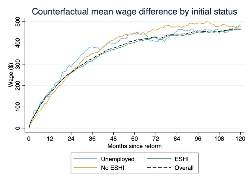
I also simulate the transition over time to the new equilibrium under universal health-
care by using the last simulated year of the benchmark model as the initial conditions of the
counterfactual simulation. I find that there is an initially sharp rise in wages as unemploy-
ment becomes more valuable and as the mass of competitive firms for each worker increases
in the absence of ESHI costs, and so over 50% of the total expected wage gains accrue by
the end of the first two years. However, wage growth quickly diminishes, and the full wage
distribution takes almost 10 years to reach the new steady state.
By contrast, in the second policy counterfactual where firms are proportionally taxed to
pay for universal healthcare in its entirety, the average wage is virtually unchanged. However,
from analysis of the full wage distribution I find that the highest quartile of earners actually
see roughly a 3% decrease in wages, while the bottom quartile experience almost a 12%
increase in their average wage due to the increased value of unemployment. This finding
suggests that in addition to providing all individuals with health insurance, this policy and
accompanying tax result in a transfer of wealth from the highest to the lowest income groups.
This redistribution of wages also occurs more quickly than in the first counterfactual, as wages
for all but the top quartile appear to reach a new steady within five years.
The result of both counterfactual analyses is more than a 2 percentage point decrease in
wage inequality in terms of Gini coefficient, with a slightly larger effect under the latter policy
change. Furthermore, despite aforementioned mechanisms within the model that would allow
for substantial inefficiencies, I find little effect of either counterfactual on unemployment, job-
to-job transitions, or joint productivity levels, suggesting that the impact of ESHI on any of
these labor market measures is negligible.
The rest of this paper will proceed as follows. In section 2, I present the relevant liter-
ature in this area; section 3 presents the full structural model; section 4 describes the data
used for estimation; section 5 details the estimation procedure and section 6 describes the
results of that estimation and their model implications; section 7 presents the counterfactual
experiments and their results; and section 8 concludes the paper and discusses potential
avenues for future research.
42 Literature
This paper is related to three primary areas of literature. First, and most closely related
is the research examining the relationship between health insurance and the labor market.
Within this area, most work has been design-based,6 but there is a smaller strand focused on
estimation of structural models of the labor market and health insurance. Fang and Shephard
(2019) estimate a search model incorporating spousal insurance and the Affordable Care Act.
Aizawa and Fang (2020) similarly estimate an equilibrium search model that incorporates
firm size and healthcare expenditure to evaluate the impact of the ACA and its various
individual components. And, similar to this paper though employing a different class of
search model, See (2019) develops an equilibrium search model and studies the overall welfare
effects of a single-payer healthcare system. See finds that welfare effects would be relatively
small, but positive, though employment would decline as reservation wages increase. The
most closely related model is that of Dey and Flinn (2005), wherein health insurance enters
utility as a binary normal good and within-firm wage dynamics result in considerable wage
dispersion among identical workers. This paper expands on this model by introducing multi-
worker firms and a greater degree of heterogeneity in order to build a richer model of wage
determination in the presence of ESHI. Specifically, modeling multi-worker firms imposes
that workers at the same firm must have the same health insurance benefits offered, which
this paper posits as an importance potential source of inefficiency in the current labor market
structure.
The second strand of literature to which this paper relates is that concerning the eval-
uation of health insurance policy reform. Of particular prevalence are those examining the
impact of the ACA, such as the aforementioned studies by Fang and Shephard (2019) and
Aizawa and Fang (2020), as well as Aizawa (2019), which studies alternative specifications
for the ACA health insurance exchange (HIX), and Aizawa and Fu (2021) which considers
cross-subsidization and risk pooling between ESHI and the HIX. This literature also includes
a large body of work evaluating the impact of the Massachusetts health insurance reform
that preceded it. Notably Kolstad and Kowalski (2012), Hackmann et al. (2012), Hackmann
et al. (2015), and Kolstad and Kowalski (2016). However, working papers by See (2019)
and Capatina et al. (2020), whose research focus is on medical expenditure shocks and their
effects on human capital accumulation over the life cycle, are some of the only examples
of papers that have touched on the potential impact of Medicare-for-all type policies. Fur-
thermore, studies of the Massachusetts health insurance reform and the ACA, which are
primarily changes in the intensive margin of employer sponsored health insurance provision,
are not readily applicable to a policy which acts on the extensive margin, eliminating ESHI
completely. This paper joins this very small body of work studying such a policy proposal
and its relationship to the labor market.
Third, this paper relates to the more general area of literature estimating structural labor
search models. Burdett and Mortensen (1998) and Postel-Vinay and Robin (2002) are the
most prominent papers in this strand of the literature, and form the basis for Aizawa and
Fang (2020) and See (2019), and Dey and Flinn (2005) respectively. In addition to these
6
See Currie and Madrian (1999) for an overview of reduced-form work on health insurance and the labor
market, and Gruber and Madrian (2004) for a review of the literature on the impact of health insurance on
labor supply and job mobility.
5papers modeling on-the-job search, wage dispersion and (in some of them) health insurance
provision, this paper relates to the class of models more generally modeling non-wage benefits.
Hwang et al. (1998) examine the impact on hedonic wage theory of search models and in
doing so develop a model of labor search where workers have heterogeneous preferences over
non-wage benefits. In this paper, I contribute to this body of research by developing a search
model of wage determination and health insurance provision that can readily be applied to
any other (discrete) non-wage benefit.
3 Model
Here I introduce a model of job search with worker and firm heterogeneity, employer-
sponsored health insurance and ESHI pre-commitment, and wage dispersion arising from
firm market power and job transition frictions. The aim of this model, based on Postel-
Vinay and Robin (2002) and Dey and Flinn (2005), is to properly characterize the rela-
tionship between the wage distribution and health insurance provision by estimating the
wage determination process in a labor market where firms make a bundled {wage, ESHI}
take-it-or-leave-it job offer having previously committed to the ESHI offer at the time of job
posting. This functions essentially as a model of wage determination with bundled non-wage
benefits, specialized to fit imputed demand for health insurance. I begin by specifying the
worker’s job search process and utility function. I then detail the firm’s objective function.
Following this, I detail the timing of the model and the wage determination process given
the model primitives, and finally, qualitatively characterize the model equilibrium.
3.1 Worker behavior
Workers search for jobs in a discrete time environment, and are heterogeneous only with
respect to their ability level, , which is drawn from some continuous distribution with cdf
F, and which is assumed to derive from some unobserved function of their human capital.
This is fixed when they enter the labor market, and their ability level determines their
unemployment “outside offer.” This is defined as the wage they could earn at some other
profession or employment opportunity (i.e. minimum wage or self employment), or from
unemployment insurance. This is modeled as a fixed offer b, and I assume an unemployed
worker receives a wage of b.
Unemployed workers are randomly matched with a firm with probability λu in each
period, and assuming it is profitable to hire the specific worker, they will receive an offer
{w, η} where w is the wage and η ∈ {0, 1} is ESHI. This model abstracts from individual
insurance premiums, and so if ESHI is provided, the worker is assumed to pay nothing for
health insurance. Employed workers match with a new firm with independent probability
λe , and the worker receives a new {w, η} offer that depends on the competition between the
two firms, detailed further in section 3.2.
Workers also have the option to purchase private health insurance H ∈ {0, 1} at price
P , if it is not provided by their job, or they are unemployed. This price is exogenously
determined by the current structure of the health insurance market and does not depend
6on the worker’s income.7 This price is assumed to be time invariant by workers. This is to
say that any change to health insurance policy, such as in my counterfactual experiments, is
assumed to enter the market as an unexpected shock.
Workers have a utility function that depends only on their income and access to health
insurance. To produce heterogeneous demand for health insurance without increasing the
parameter space, I assume diminishing marginal returns to income, u(Y ) with u00 (Y ) < 0,
with a separable, constant marginal utility of health insurance. This results in an increasing
marginal rate of substitution of health insurance for income, with the effect that stochas-
tically, higher ability workers will forgo more wages in exchange for health insurance than
low ability workers. Workers with wage w, health insurance offer η and individual health
insurance purchase decision H then have flow utility
v(Y, H, η) = u(Y ) + α(η + (1 − η)H)
s.t. Y = T (w) − (1 − η)P H
where income Y is equal to the after-tax8 wage T(w) minus the price of health insurance
in the event it is not provided and the individual chooses to buy it, and α is the constant
utility of health insurance, which is the same whether purchased privately or provided by
the employer. This is the sole manner in which health insurance enters worker utility, as I
abstract from any direct health implications of access to healthcare for the sake of tractability.
Since the primary goal of this paper is to understand the firm’s wage offer response to policy
changes, the structure of individual health insurance preferences is not so important, only
that, broadly speaking, workers like to have it, and so firms can pay them less in exchange
for providing it.
Of course, introducing health insurance as a simple dummy variable that enters utility
as a normal good perhaps requires additional justification. Most of the literature treats
health insurance as, fittingly, insurance, where individuals face some random distribution
of healthcare cost shocks and having health insurance mitigates or eliminates that risk.
However, underlying these models is the assumption that the value of health insurance
is solely a financial one, whereas a large body of empirical literature has found that the
uninsured receive fundamentally different healthcare.9 So, it is both easier to estimate and
perhaps equally representative of the true value of health insurance to workers to estimate
an indirect utility parameter for having it or not.
Returning to worker behavior, employed workers continue to match with firms at the
same rate, and, if a new offer gives higher utility, can choose to switch firms at no cost.
Searching for jobs is assumed to be costless to the worker as well. Finally, employed workers
face an exogenous job destruction rate δ.
7
In the baseline model, I do not allow for individuals to receive health insurance through Medicaid or
Medicare, and those individuals are excluded from the estimation sample. Note however, that only persons
age 65 or above qualify for Medicare, and very few employed individuals qualified for Medicaid prior to the
ACA, and so excluding these cases should not significantly bias my results.
8
This tax function is relatively inconsequential as it only serves to change the interpretation of α from
pre-tax to post-tax relative wage increase. However, as income tax is a realistic feature of the market and
easy to implement, I estimate a tax function following Heathcote et al. (2017). Details for this tax function
are included in Appendix A.
9
See for example Monheit et al. (1985) and Kolstad and Kowalski (2012).
73.2 Firm behavior
Similar to workers, firms are heterogeneous only in their productivity parameter, ρ, and
receive revenue from hiring a worker of ability level equal to ρ. This means that firms
value higher ability workers, and higher productivity firms value an identical worker more
than lower productivity firms. I assume a continuum of firms with some distribution G of
productivity levels. Since all firms must be able to at least match the unemployment benefit
in order to hire any worker, I assume a lower bound ρ = b, as is standard in this class of
models.
Firms post jobs at no cost, and hire a continuum of workers at some rate determined
by workers’ match probabilities. The exact matching rate for each firm is irrelevant to the
model equilibrium as I do not track firm size and I assume profit is additively separable
across workers. The only meaningful capacity in which firms are multi-worker is that, prior
to matching, each firm must decide whether or not to offer health insurance to all potential
workers. Each match results in an optimal take-it-or-leave-it wage, ESHI offer upon meeting
the worker that depends on the worker’s productivity level and current employment status.
This commitment mechanism for health insurance is designed to approximate the reality
that wages are determined on an individual level upon interviewing job candidates, but
health insurance must typically be offered to all workers with analogous job descriptions.
Modeling multi-worker firms in this way is a simplifying assumption to avoid more explicitly
incorporating firm size, while introducing a realistic inefficiency in firms’ ability to adjust
offer bundles to fit individual workers.
If firms provide health insurance, they pay a fixed rate ψ per worker per period. So a
firm with productivity level ρ employing a worker of ability with health insurance offer
η ∈ {0, 1} has flow profit
π = ρ − w − ψη
The firm will offer the worker the lowest possible wage such that this worker accepts the
offer. However, if this wage is such that profit is negative, given the pre-committed choice to
provide ESHI or not, the firm will be unable to hire this worker and profit is equal to zero.
3.3 Timing and wage determination
The timing of this infinite horizon model is as follows. In the pre period, firms observe the
unemployment rate and the distribution of worker ability, and each firm makes a choice of
whether to offer health insurance in their job postings. These firms then enter the market
randomly according to workers matching rates. Each worker starts unemployed at the time
they originally enter the market. The timing at which each worker enters the market is
assumed to be random, and it is assumed that the distribution of worker abilities entering
the market is time-invariant. I assume the market is in a steady state10 and workers enter
10
There is an inherent initial conditions problem in simulating this class of models as without explicitly
modeling age we cannot observe how long workers have been in the market prior to the sample period. To
overcome this, I simulate an initial period in which workers are randomly assigned to unemployment or a
firm of random productivity level according to the unemployment rate and distribution of ρ, and I assume
that employed workers in this period receive their unemployment indifferent wage. I assume the data are
in a steady state, and so I then simulate a 48 months of this labor market and use the final month as the
8each period with their employment and ESHI status determined from the previous period.
Workers then choose whether to buy health insurance if it has not been provided, given their
wage. Workers’ flow utility is then realized. After realizing their flow utility, some employed
workers exogenously lose their jobs with probability δ and enter the next period unemployed.
Workers who entered the period unemployed match with a firm with probability λu . Each
firm observes the employment status and ability level of their matched worker, and, if profit
(conditional on their ESHI decision) is non-negative, offers the worker a {w, η} bundle. Firms
offer unemployed workers the lowest wage that makes them indifferent between remaining
unemployed and working at the matched firm. When indifferent, the unemployed worker is
assumed to accept the offer. If this wage is such that profit is negative, no offer is made and
the worker remains unemployed.
The remaining employed workers match with a new firm with probability λe . A new
match is made, the new firm and the current firm engage in Bertrand competition for the
worker, given their respective productivities and ESHI policies. Whichever firm is able to
offer the combination of wage and ESHI that gives the worker the highest utility will hire
the worker, and the worker will receive a wage that makes them indifferent between the old
firm and new firm. If both firms have the same ESHI policies, the worker will choose the
firm with the highest productivity level. These workers enter the next period employed at
the winning firm and with the wage and ESHI status determined from this competition.
Employed workers who do not match with a new firm, do not lose their job, or match
with a firm that cannot make a competitive offer given their current wage and insurance
status, enter the next period with their wage and insurance status unchanged.
Each period, it is assumed that the labor market demographics are in a steady state. Of
course, each period some workers permanently leave the market (i.e. retirement or death),
and others enter the labor force, but because I assume ability and match productivity dis-
tributions are independent of age or market time period, the entry and exit of workers from
the labor force is observationally equivalent to infinitely lived agents who simply lose their
jobs randomly and start over in the wage distribution. In this way I abstract from any
life cycle wage growth, and all wage growth is instead assumed to come from repeated on
the job matching with higher productivity firms. This is done primarily for computational
efficiency, as it reduces the number of states that must be kept track of, but also because the
data available tracks individuals for only four years, and so a full life-cycle implementation
is infeasible.
3.3.1 Value functions
Given these timing assumptions, I can write down the worker’s value functions. For a worker
with given ability level the value of being unemployed in any period t is equal to
U () = max u(T (b) − P H) + αH
H∈{0,1}
n o
+ β (1 − λu )U () + λu Eρt+1 Eηt+1 (ρt+1 ) V (, wt+1 , ρt+1 , ηt+1 ) (1)
initial conditions for my estimation period.
9with discount factor β ∈ (0, 1), taking expectation over possible firm productivity ρt+1 draws
and the probability of being offered offered health insurance ηt+1 , which will depend on ρt+1 .
The worker has perfect information regarding the determination of wages, which will depend
on the worker’s time-invariant ability level, current employment status, and the productivity
of the firm with which she is matched, and the ESHI probabilities, which depend only on
the matched ρt+1 productivity firm. Note that flow utility for unemployed workers is the
same in every period, and the expectations over ρ and η will be the same for all unemployed
workers, and so U () is time invariant and only depends on the workers ability level.
Similarly, the value to a worker of being employed by a firm with productivity level ρt ,
at wage wt , and with ESHI provision ηt is equal to
n
Vt (, wt , ρt , ηt ) = max u(T (w) − (1 − η)P H) + α(η + (1 − η)H) + β δU ()
H∈{0,1}
+ (1 − δ) λe Eρ0 Eηt+1 (ρt ,ρ0 ) Vt+1 (, wt+1 (ρt , ρ0 ), ρt+1 (ρt , ρ0 ), ηt+1 (ρt , ρ0 ))
o
+ (1 − λe )Vt+1 (, wt , ρt , ηt ) (2)
where again the wage next period, in the event of a match, depends on the productivity of
the current firm and the new firm productivity draw ρ0 . Next period’s firm productivity ρt+1
will depend on the relative productivities of current firm ρt the matched productivity ρ0 ,
and their respective ESHI offers. Otherwise, if the worker experiences job destruction with
probability δ, they become unemployed next period, whose value depends only on . If the
worker does not lose her job and receives no alternative offer, she receives the same wage
and ESHI offer from the current ρt firm next period.
As stated above, wage determination follows a very particular process. Workers have
no bargaining power, in the manner of Postel-Vinay and Robin (2002). Instead, firms bid
against each other, and the worker gets her indifference wage. The result of this feature of
the model, in addition to the desired wage growth and dispersion effects, is that wages are
deterministic given current productivity ρ, new matched productivity ρ0 , and the two firms’
pre-committed ESHI offers η and η 0 respectively. Borrowing notation from Postel-Vinay
and Robin, I represent the unemployed and employed indifference wage, respectively, that
workers can expect by φ0 (, ρ, η) and φ(, ρ, ρ0 , η, η 0 ). Since the firm will offer the lowest
wage possible to incentivize the worker to accept the offer, for unemployed workers, this
wage satisfies the following:
φ0 (, ρ, η) = w∗ s.t. U () = V (, w∗ , ρ, η) (3)
Similarly, for employed workers, the wage that incentivizes the worker of ability level to
switch from a firm of productivity ρ to a firm of productivity ρ0 satisfies
φ(, ρ, ρ0 , η, η 0 ) = w∗ s.t. V (, w̄(ρ, η), ρ, η) = V (, w∗ , ρ0 , η 0 ) (4)
where w̄(ρ, η) is the maximum wage offer the losing firm can make given its choice of η.
Importantly, the job transition will depend on the respective productivities and health in-
surance policies. In section 3.2, I mention that firms will make an offer only if profit is
non-negative. The result is that though it is probable workers will choose to accept the
10indifference wage offer from the higher productivity firm, cases may arise where the relative
productivity gains of the more efficient firm are not sufficient to cover the cost of outbidding
the lower productivity firm, if the higher productivity firms has committed to offering health
insurance and the lower has not. This can produce productivity-inefficient job transitions in
some cases. I discuss this explicitly in section 3.4.
Observing these indifference wages and anticipating the ESHI probabilities of competing
firms, a firm with productivity level ρ, committed to ESHI provision choice η has a value of
matching with an unemployed, productivity level worker of
(
n
Jtu (, ρ, η) = 1π>0 π(, ρ, φ0 (, ρ, η), η) + β(1 − δ)
)
o
u
(1 − λe )Jt+1 e
(, ρ, η) + λe Eρ0 Jt+1 (, ρ, ρ0t+1 , η, ηt+1
0
) (5)
where J e (, ρ, ρ0 , η, η 0 ), the value of matching with a worker currently employed at another
firm with productivity ρ0 and ESHI provision choice η 0 , is equal to
(
n
Jte (, ρ, ρ0t , η, ηt0 ) = 1π>0 π(, ρ, φ(, ρ0t , ρ, ηt0 , η), η) + β(1 − δ)
)
o
e
(1 − λe )Jt+1 (, ρ, ρ0t , η, ηt0 ) + λe Eρ0t+1 Jt+1
e
(, ρ, ρ0t+1 , η, ηt+1
0
) (6)
If the matched worker is unemployed, provided the firm can afford to hire her (π > 0), the
firm realizes flow profits. The next period, the firm expects that, provided the job is not
exogenously destroyed, this worker will match with another firm with probability λe . If the
worker does not match with another firm, this firm gets the same value J u in the next period.
If the worker does match with another firm, this firm must compete with the new firm and
will get the employed match value J e of this worker, taking the expectation over all possible
productivity levels of the competing firm.
This employed value functions similarly, but will depend on φ(, ρ0 , ρ, η 0 , η), i.e. the wage
the firm needs to offer the worker to make her indifferent between staying at the current
firm and switching. If this wage results in negative profits, the firm loses the worker and the
job is destroyed. If the firm hires the worker, then with probability (1 − λe ) they keep the
worker at the same wage next period, and with probability λe the worker matches with a
new firm and this firm receives the value of competing with the new firm.
Given these value functions, in the initial period (period zero) the firm’s probability of
offering health insurance is determined by solving
max E u()J u (, ρ, η) + (1 − u())Eρ0 | Eη0 |ρ0 J e (, ρ, ρ0 , η, η 0 ) − 1η=1 ξ (7)
η∈{0,1}
where u() is the unemployment rate of workers of ability level , which will be determined
by δ, λu , and also the ability distribution and firms’ ESHI policies. Note that the proba-
bility a worker is currently employed at a given productivity level firm will depend on that
11worker’s ability level since non-monotonicity of productivity in job transitions means and
ρ distributions are not independent given current employment.11 This holds true only in
period zero, as once a firm has employed a given ability level worker, the probability of
that worker meeting a firm of productivity level ρ0 is independent of the worker’s ability.12
Here I also introduce ξ, a stochastic cost shock introduced primarily to aid in equilibrium
convergence. This can be justified as a randomized “health plan participation fee” that is
a sunk cost after period zero, and has the effect of randomizing firms’ ESHI decision such
that η(ρ) ∈ [0, 1] becomes a continuous function. I discuss this further in section 5.
3.4 Description of equilibrium
Due to the complexity of the model given multi-worker firms with committed health in-
surance provision decisions, an analytical solution is infeasible. As such, I solve the model
computationally using the algorithm specified in section 5.3. However, here I provide some
qualitative features of the equilibrium given the model’s design and the calibrated parameter
estimates.
Equilibrium is defined in this model as the fixed point of the mapping between wage
function φ0 (, ρ, η(ρ)) and φ(, ρ, ρ0 , η(ρ), η 0 (ρ0 )), and ESHI provision probability function
η(ρ), which is equal to the probability that the solution to equation (7) is equal to one,
given the distribution of ξ. Since the indifference wages are deterministic, given a fixed η(ρ)
probability function, φ0 and φ can be directly calculated using value function iteration.
In equilibrium, this η(ρ) is strictly increasing in ρ as higher productivity firms offer
higher wages, holding constant, and the marginal rate of substitution of income for health
insurance increases with wages. This is also at least partly due to the fact that higher
productivity firms earn higher revenue from each type of worker and so are more likely to be
able afford the cost of providing health insurance. Similarly, the provision of health insurance
has the potential to create an unemployment wedge amongst low productivity workers and
firms as the cost of ESHI may exceed their joint productivity. However, in the simulated
data this wedge appears to be of limited importance as the difference in the unemployment
rate with the removal of ESHI is insignificant.
Another important feature of the model is that in equilibrium, though firms are able
to decrease wages in exchange for providing health insurance, it should be the case that,
stochastically, higher wage jobs are more likely to provide health insurance, since dη(ρ) dρ
> 0.
Indeed, in the simulated data, with roughly 85% of jobs providing health insurance, wages
at jobs with ESHI are 74% higher than wages at jobs without ESHI.
Finally, it should be the case that in the event of a change to health insurance policy, i.e. a
change in P , there should be some delay between the beginning of the policy and convergence
11
Without health insurance, as in Postel-Vinay and Robin (2002), workers will always move from ρ to ρ0
given that ρ0 > ρ. The results is that, though the expected productivity level of a matched firm increases with
employment duration, this is equally true of all workers, and so E(|ρ) = E(), and vice-versa. However,
with ESHI, if for example the same ρ does not provide health insurance but ρ0 does, some workers of low
ability may not be productive enough for ρ0 to attract them away from ρ, given the cost of ESHI, and so for
some particular ability level ˜, P ( = ˜|ρ0 ) = 0 and so E(|ρ0 ) 6= E().
12
The worker’s offer, and therefore the match value is dependent on the worker’s ability, but the worker can
still “match” with any firm. This is to say that λu and λe are independent of worker or firm productivities
and if gainful employment cannot be produced, both sides are out of luck until the following period.
12to the new steady state equilibrium wage distribution as, generally speaking13 ,wage increases
require meeting with a new (and competitive) firm. Initial offers out of unemployment should
see the quickest increase as the value of unemployment as an outside option increases with
more affordable private insurance. The exact degree of this change however will depend
on the relative value of the insurance and the cost to firms of providing it, as well as the
average duration of employment. This is because as workers remain employed and receive
additional offers, their wage rises closer to the level of their joint productivity with the
firm. Conversely, the percentage of this surplus allocated to workers decreases as the job
destruction rate increases.
4 Data
To estimate this model, I primarily utilize the 2008 panel of the Survey of Income and
Program Participation (SIPP). The SIPP contains monthly data on individual labor market
outcomes and health insurance coverage, as well as demographic and household composition
variables. These data are collected during interviews conducted every four months, up to
twelve times, so individuals may be tracked for up to four years. I use the core module
of this data14 containing detailed labor market variables including earnings, employment
status, number of weeks worked, industry of the job worked, as well as whether the individual
changed jobs during each month of the four month survey period. Health insurance status
is recorded as well, including whether insurance was provided by the employer or privately
purchased, or came from Medicare or Medicaid, and whether the individual was covered
under their own insurance plan or someone else’s.
For estimation, I restrict the sample considerably to match the labor market environment
detailed in the model. I retain only individuals participating fully in the labor force for the
full 48 months, and who only receive health insurance from an employer or private purchase.
For this, I drop individuals below 18 years of age and above 64 years of age, any individual
enrolled in school, as well as any individual who receives Medicaid, Medicare, or obtain
health insurance through a family member. I also drop from the sample any individual who
is not observed to work at any point during the four year sample period. I further remove
individuals working in the public sector, or self-employed, as these types of jobs do not fit
the ESHI incentive structure in the model.15 I also restrict the sample to individuals not
receiving social security income and not involved with the military. To remove some likely
outliers in income or program participation, while continuing to maintain a good deal of
worker heterogeneity in productivity, I retain only individuals who have completed at least a
13
In section 7, I discuss the exception in the first period, where workers lower in the ESHI wage distribution
for whom unemployment has become preferable to employment at the current firm and wage will be able to
renegotiate and raise their wage back to the indifference level.
14
The SIPP contains a core module, with the primary variables on labor market outcomes and health
insurance coverage, as well as other public program utilization (i.e. food stamps, etc.), in addition to a
topical module, with various other topics, including some expenditures such as health insurance premiums
or tuition, collected annually. I do not use the topical module as the model abstracts from worker premiums
for ESHI, but this data could be used for such an extension to the model in the future.
15
Public sector jobs are overwhelmingly likely to provide health insurance, and do so for reasons related
to public policy rather than profit maximization.
1310th grade education. Finally, I restrict the sample to those individuals who are in the data
for the full four years, given all of the above restrictions, so as to obtain a balanced panel.
This leaves an estimation sample consisting of 5,014 individuals tracked over 48 months for
a total of 240,672 observations.
In addition, since the SIPP does not collect information on employers beyond the industry
and a longitudinal identifier, I use data from the Kaiser Family Foundation Employer Health
Benefit Survey (KFF) from 2009-2012, the years corresponding to those present in the SIPP
panel, to obtain estimates for employer sponsored health insurance premium costs. The KFF
contains annual data, from firms in the private and public sector, on firm characteristics such
as size, industry, and employee demographics, as well as, for my purposes, health insurance
premiums paid. I restrict the sample to firms in the private sector, and utilize this data only
to estimate the employer monthly premium parameter ψ.
4.1 Summary statistics
Summary statistics for the 2008 SIPP panel are presented in Table 1 below. As this sample
is restricted to individuals that appear in all 48 months, the average months employed is
quite high at 44.84, despite 30.8% that experience at least one month of unemployment. Just
under half of the individuals are ever observed switching jobs, defined as starting a new job
either out of unemployment or from a different employer, data for which is recorded using
distinct employer IDs. Similarly, individuals are observed to transition between jobs at a
rate of only 1.4%.
From the insurance coverage data, 17.9% of the sample are uninsured, which matches
closely with the Kaiser Family Foundation’s reported national averages, once Medicaid,
Medicare, and military personnel are excluded. 80.1% of the sample receive insurance
through their employer (and 85% of employed individuals), and less than 2% purchase insur-
ance privately. It can also be seen that the average monthly wage at jobs providing health
insurance is almost twice that of jobs without ESHI. This is a larger discrepancy than is
reported in much of the literature, and I have little to offer as an explanation as to why this
is the case here. This is also the data trend that has proved the most difficult to closely
replicate in model simulations.
5 Estimation
In this section, I detail the estimation procedure used to obtain parameter estimates. I
estimate the model using a two step process. In the first step, exogenous model primitives
and several structural parameters are estimated from observed sample means. In the second
step, the remaining structural parameters are estimated using the iterative algorithm detailed
in section 5.3. To begin with however, I will detail the identification argument and the
assumptions necessary to overcome data limitations.
14Table 1: SIPP 2008 Summary Statistics
Selected Sample
Variable Mean S.D.
Employment
Months employed 44.84 7.85
Ever unemployed .308 .462
Ever switch jobs .459 .498
New job in the month .022 .146
Job-to-job transition .0140 .117
Exited unemployment .142 .349
Became unemployed .0103 .101
Insurance Coverage
Uninsured .168 .374
ESHI .813 .390
Privately Insured .019 .137
Earnings
UI benefits 1,171.11 590.87
Wage 4,104.98 2368.02
Wage, ESHI 4,427.39 2,351.31
Wage, uninsured 2,274.08 1,453.84
N = 5,014
5.1 Identification and assumptions
I begin with some simplifying assumptions not essential for identification but whose implica-
tions either aid in comprehension or substantially reduce computation time (or both). First,
though the results should extend to a generalized concave utility function, the precise shape
of the utility of income does not qualitatively alter the functioning of the model,16 and so I
assume log utility of income to eliminate an estimation parameter.17 Quantitatively, results
may change slightly in the presence of very high concavity, but log utility remains firmly
16
This is true of incorporating an income tax function into the model as well. Including taxes changes the
interpretation of α from pre-tax to post-tax percent marginal income increase. But with or without taxes in
the model, the pre-tax wage value of health insurance remains unchanged.
17
This also speeds up computation slightly as Julia’s built in log function evaluates more quickly than, for
exapmle, a CRRA functional form with risk aversion parameter γ = 1.1. In tests this reduced the time it
takes to solve the model by about 40% and did not significantly alter the results.
15within the bounds of the literature’s estimation of reasonable risk aversion.18 Similarly, I
normalize the unemployment benefit b to 1, since the level of this value is inconsequential,
and normalizing it so allows me to identify the distribution of directly from the sample
distribution of unemployment “wages.” I also parameterize the productivity distributions for
both the worker and firm, F ∼ log N (µ , σ ), G ∼ log N (µρ , σρ ) as these distributions must
be positive and together characterize wage distributions, of which lognormal distributions
typically provide a good approximation. Note, however, that since all observed values of
ρ must be above b, I assume instead ρ − b ∼ log N (µρ , σρ ). With these assumptions, my
parameters of interest reduce to {α, µ , σ , µρ , σρ } along with exogenous firm health insur-
ance costs ψ, the similarly parameterized distribution of cost shock ξ ∼ log N (µξ , σξ ) where
I assume µξ = 0, and the transition parameters δ, λu and λe . Following the work of many
before me, and deriving from Flinn and Heckman (1982), I do not attempt to separately
identify the discount rate β, and instead fix it at 0.995, which gives an annual interest rate
of 6%.19
I estimate these parameters using a two-step process whereby exogenous parameters
{ψ, δ, λu } are identified from sample means in the data. The assumption that any employer
will be able to hire any worker out of unemployment, and that workers will accept any
offer that makes them at least indifferent, allows me to estimate λu from the mean monthly
probability of transitioning out of unemployment in the SIPP data.20 The job destruction
rate δ is also set equal to the mean monthly probability of becoming unemployed observed
in the data. The firm cost of providing health insurance is estimated using the KFF data,
whereby monthly premium ψ is set equal to the weighted sample mean monthly premium
cost per employee, while the cost shock parameter σξ is estimated in the second step.
The identification of the distribution of firm productivity, the utility of health insurance,
and the variance of the unobserved cost shock require more justification. The parameter-
ization of the productivity distribution to a log normal coupled with fixed job transition
rates and fixed parameterized distribution of makes the employed wage distribution sam-
ple moments sufficient to identify µρ and σρ . This leaves α to be estimated as the primary
determinant of wage depression resulting from health insurance, and σξ as a partial de-
terminant of the ESHI coverage rate. An increase in α increases the ESHI provision rate
as providing health insurance becomes more profitable with larger compensating wage de-
creases, but decreases the difference between ESHI and non-ESHI mean wages as the former
wages are increasingly depressed in exchange for health insurance, while the latter wages
must be increased to offset the lack of ESHI. An increase in σξ holding other parameters
constant decreases the insurance provision rate since providing it becomes more costly on
18
See Chetty (2006) for discussion of reasonable risk aversion parameters in labor supply models. He finds
a mean estimate across studies of γ = 0.71, and estimates bounds between 0.15 and 1.78. As such, γ =1
is selected for this paper for its computational expediency and the interpretability it lends to the estimated
value of α.
19
This is higher than the rate of wage growth observed in my sample and the BLS reported interest rate
during this period, however, with monthly data, increasing β above 0.995 begins to substantially slow down
the convergence of the value function. Increasing the interest rate while remaining at a reasonable value
observed in much of the literature served to decrease computation time of the full model equilibrium by
roughly 50% and did not impact the goodness of fit of the estimated model.
20
I previously discussed a potential unemployment wedge that would cause this assumption to fail, but
given that I do not find such an inefficiency from the estimated parameters, this assumption seems justified.
16average, but also decreases the insurance-non-insurance wage gap, as higher variance in ex-
pected costs increases the probability that lower productivity firms provide health insurance
and decreases the probability that higher productivity firms provide it. These compara-
tive statics allow me to separately identify these parameters using moments concerning the
difference in the wage distribution for jobs with and without ESHI, and the overall health
insurance provision rate from the SIPP data.
5.2 First step
In the first step I estimate a number of model parameters from observed sample means.
As stated above, I am able to estimate λu directly from the observed transition rates out
of unemployment. The percentage of unemployed individuals in each month that switch
to employed in the following month is averaged over the 48 month sample and assumed
to be constant over the sample period. An analogous strategy is used to estimate the job
destruction rate. Similarly, ψ is fixed at the average monthly cost per employee of providing
health insurance reported in the KFF data, weighted by the SIPP sample percentages of
workers on individual vs. family insurance plans. µ and σ are then estimated by fitting a
lognormal distribution to the observed unemployment income in the SIPP selected sample.
5.3 Second step estimation algorithm
Fixing the first step parameters at their point estimates, I proceed to estimate the remaining
parameters using the simulated method of moments (SMM). Broadly, this consists of solving
the model for a given set of parameters, simulating a dataset from the model solution, and
using this dataset to compute model moment equivalents. These moments take the place of
model moments that are an analytical function of the parameters in the generalized method of
moments (GMM). I use cross-sectional moments on wages, insurance provision, employment,
and the interaction of these variables to compute the SMM objective function, and solve for
the model parameters that minimize this objective using the Nelder-Mead algorithm. If m
is the vector of targeted moments, and θ is the vector of model parameters let
h i
M (θ) = m − E[m|θ] (8)
and the objective function is constructed as
min M (θ)0 W M (θ) (9)
θ
where W is a weighting matrix consisting of the inverse of the variance of the moments,
adjusted individually to weight the moments more essential to obtaining reliable counterfac-
tuals. To generate M (θ), the model is solved using the following algorithm:
1. Given distribution parameters, discretize the worker and firm productivity distribu-
tions.
2. Compute unemployment value function U (), since this does not depend on the wage
distribution at equilbrium.
173. Initialize the employment indifference wage function φ(, ρ, ρ0 , η, η 0 ) and ESHI function
η(ρ). The initial guess for the wage function sets the wage necessary to switch equal to
the maximum wage the losing firm can afford to the pay the worker. The initial guess
of η(ρ) doesn’t matter so much, as this adjusts quickly, and is set to 0.5 for all firms.
4. Iterate on the indifference wage function and η(ρ) to find the fixed point
(a) Given productivity distributions and initial guesses , solve workers’ value func-
tions.
(b) Given value functions solve for indifference wages, with and without ESHI, for
unemployed, and for employed given current productivity employer, φ̂0 (, ρ, η)
and φ̂(, ρ, ρ0 , η, η 0 ).
(c) Given indifference wages, solve for ESHI probability η̂(ρ) at each ρ of the dis-
cretized distribution.
(d) Evaluate d(φ0 , φ̂0 ), d(φ, φ̂) and d(η(ρ), η̂(ρ)), where d() is a distance metric. If
these are less than the specified tolerance level, the equilibrium has converged. If
not, update each function according to φ0 = ωφ0 + (1 − ω)φ̂0 , φ = ωφ + (1 − ω)φ̂,
and η(ρ) = ωη(ρ) + (1 − ω)η̂(ρ), for ω ∈ (0, 1), and return to step 4(a). Repeat
until convergence.
5. From the computed model equilibrium, simulate job histories for N individuals over T
months to reasonably match the horizon of the true data.21
6. Evaluate the moment function and update parameter guesses. Repeat until conver-
gence criterion are met.
This method is used to obtain point estimates of the model parameters. The standard
errors of these parameters are estimated in the manner of GMM, where if M(θ) = E[ ∂M (θ)
∂θ0
]
0
is the gradient matrix of the moment conditions evaluated at θ̂, and if Ω = E[M (θ)M (θ) ]
is
√ the variance-covariance matrix of the moment conditions, then the asymptotic variance of
n(θ̂ − θ) is
−1 −1
M(θ)0 W M(θ) M(θ)0 W ΩW M(θ) M(θ)0 W M(θ)
and the standard errors are the square root of the diagonal elements of this matrix divided by
n. The estimator of the asymptotic variance cannot be simplified since W cannot be said to
be a consistent estimator of the efficient waiting matrix. Note also that, as in Petrin (2002)
and Aizawa and Fang (2020), I assume that Ω is a block diagonal matrix since different
moments are derived from different sampling and sub-sampling processes.
21
In this case, N is set to 5000 and T is set to 96, of which the first half are thrown out and the final 48
months are used to calculate simulated moments. This is done to overcome the initial conditions problem that
arises in simulating steady state models such as this one. I have experimented with alternate pre-estimation
time horizons and after any number past 48 months (i.e. 96 total) the results were unchanged.
18You can also read