Life Insurance and Subsistence Consumption with an Exponential Utility - MDPI

Page created by Darren Bowen
 
CONTINUE READING
Life Insurance and Subsistence Consumption with an Exponential Utility - MDPI
mathematics

Article
Life Insurance and Subsistence Consumption with an
Exponential Utility
Ho-Seok Lee

                                           Department of Mathematics, Kwangwoon University, Seoul 01897, Korea; hoseoklee@kw.ac.kr

                                           Abstract: In this paper, we derive an explicit solution to the utility maximization problem of an
                                           individual with mortality risk and subsistence consumption constraint. We adopt an exponential
                                           utility for the individual’s consumption and the martingale and duality method is employed. From
                                           the explicit solution, we exhibit how the mortality intensity and subsistence consumption constraint
                                           affect, separately and together, portfolio, consumption and life insurance purchase.

                                           Keywords: life insurance; subsistence consumption; portfolio selection; exponential utility; martin-
                                           gale method

                                           1. Introduction
                                                 In portfolio selection problems, considering some constraints create difficulties in solving
                                           the relevant optimization problems but increase the realism. Borrowing constraints restrict
                                           individual’s financing only up to a partial amount of the individual’s human capital or do not
                                           allow any amount of borrowing. Borrowing constraints lead individual to reduce investment
                                           in the risky asset and to decrease consumption. Mathematical finance literature that mainly
                                           focuses on the effects of partial borrowing constraints on optimal decisions for individuals
         
                                    includes [2,3,5,15–17]. References [12,14] consider the case where an individual cannot borrow
                                           against future labor income at all, and especially the last one investigates how the borrowing
Citation: Lee, H.-S. Life Insurance
                                           constraints and job choice flexibility affect on portfolio selection and consumption.
and Subsistence Consumption with
                                                 Subsistence consumption constraints imply that an individual must consume at least
an Exponential Utility. Mathematics
2021, 9, 358. https://doi.org/
                                           a minimum level of consumption rate, for example a minimum level of consumption rate
10.3390/math9040358
                                           required to keep up life. Subsistence consumption constraints also have significant effects on
                                           the optimal decisions for individuals. Restrictions on subsistence level of consumption also
Academic Editor: Antonella Basso           make an individual’s portfolio strategy less aggressive and leads decrease in consumption.
Received: 10 January 2021                  References [4,18,19] study an infinitely lived individual’s consumption, portfolio strategies
Accepted: 8 February 2021                  while considering subsistence consumption constraints. Working individuals who face subsis-
Published: 11 February 2021                tence consumption decide retirement wealth levels differently from those who do not have
                                           such restrictions, as the analytical results from [6,9–11,13] imply.
Publisher’s Note: MDPI stays neu-                This paper is an extension of literature that investigates how the existence of subsis-
tral with regard to jurisdictional clai-   tence consumption constraints affect individual’s lifetime investment and consumption
ms in published maps and institutio-       strategy. We assume an exponential utility function for consumption and consider an
nal affiliations.                          individual’s mortality risk by adopting an exponential distribution for the death time.
                                           Based on martingale and duality method, we derive optimal consumption, portfolio, and
                                           life insurance strategies explicitly and exhibit how the force of mortality and subsistence
Copyright: © 2021 by the authors. Li-
                                           level of consumption affect, separately and together, on the individual’s decision mak-
censee MDPI, Basel, Switzerland.
                                           ing. Numerical illustrations reveal that a strong force of mortality and a high subsistence
This article is an open access article
                                           level of consumption result in reduced consumption and small investment in the risky
distributed under the terms and con-       asset. Numerical illustrations also show that life insurance demand increases with force
ditions of the Creative Commons At-        of mortality and decreases with subsistence level of consumption. However, the effect of
tribution (CC BY) license (https://        subsistence consumption constraint on demand for life insurance seems to be marginal. We
creativecommons.org/licenses/by/           also observe that an individual with a large coefficient of absolute risk aversion purchases
4.0/).                                     more life insurance.

Mathematics 2021, 9, 358. https://doi.org/10.3390/math9040358                                        https://www.mdpi.com/journal/mathematics
Mathematics 2021, 9, 358                                                                                           2 of 10

                                This paper proceeds as follows. Section 2 introduces financial and life insurance mar-
                           kets and our model. The utility function and the optimization problem we seek to solve is
                           defined in Section 3, followed by Section 4 where we use the martingale and duality method
                           to obtain explicit solution to the optimization problem. Section 5 illustrates numerical ex-
                           amples from which we examine effectcs of force of mortality and subsistence consumption
                           constraint on an individual’s decision making, and Section 6 sums up and concludes.

                           2. The Market and Model
                                  We assume that the individual participates in the financial market and can hedge
                           the mortality risk. The financial market is simply consists of a risky asset and a riskless
                           asset (money market account). The risk factor of the risky asset and that of mortality are
                           uncorrelated. Denote by (Wt )t≥0 a standard Brownian motion for a given probability space
                           (Ω, F , P). The individual’s death time τ has an exponential distribution with the parameter
                           λ > 0, called mortality intensity or force of mortality. The probability density function
                           f τ (t) of τ is given by
                                                                f τ (t) = λe−λt , t ≥ 0.
                                Denote by F , (Ft )t≥0 the P-augmentation of filtration generated by the standard
                           Brownian motion (Wt )t≥0 and 1{t≤τd } . In financial markets, there exist a riskless asset and
                           a risky asset whose prices are Mt and St at time t, respectively.
                                At time t ≥ 0, the risky asset price St follows a log-normal distribution as follows

                                                                  dSt /St = µdt + σdWt ,

                           where µ > 0 and σ > 0. The risky asset’s mean rate of return per unit time, µ, and its
                           volatility σ are assumed to be constants. The riskless asset price Mt is assumed to follows

                                                                      dMt /Mt = rdt,

                           where r < µ is the risk free interest rate and it is also constant.
                               Let πt be the amount of money invested in the risky asset. If
                                                            Z t
                                                                  πt2 dt < ∞ for all t ≥ 0 a.s.,                      (1)
                                                             0

                           and if π , (πt )t≥0 is F- adapted, we call π a portfolio process. In this paper, we consider
                           the case where the individual has a subsistence consumption constraint. We call the mini-
                           mum consumption rate the individual must consume the subsistence level of consumption
                           R > 0. If ct is the consumption rate at time t, it is satisfied that

                                                                    ct ≥ R, 0 ≤ t ≤ τ.

                                If                 Z t
                                                         ct dt < ∞, ct ≥ R, for all 0 ≤ t ≤ τ a.s.,
                                                     0

                           and c , (ct )t≥0 is F, we call c , (ct )t≥0 a consumption process.
                                 We assume that life insurance contracts we are considering cover mortality risk and
                           they are actuarially fair. We denote by pt and Lt the instantaneous life insurance premium
                           rate paid by the individual and insurance benefit paid by the insurer, respectively. Since
                           the life insurance contracts are fair, the insurance premium paid by the policyholder during
                           the infinitesimal time dt is equal to the insurance benefit multiplied by the probability of
                           death during the infinitesimal time dt. Thus we have

                                                                         pt = λLt ,
Mathematics 2021, 9, 358                                                                                           3 of 10

                           and the bequest Bt received by the individual’s heir is given by

                                                            Bt = Xt + Lt = Xt + pt /λ,                                (2)

                           where Xt is the wealth level. The individual’s labor income rate is constantly y > 0. Thus,
                           we have the following wealth level process

                                                     dMt                           dSt
                                     dXt = ( Xt − πt )     + (y − ct − pt )dt + πt
                                                      Mt                           St
                                          = {rXt + y − ct − pt + πt (µ − r )}dt + σπt dWt
                                          = {(r + λ) Xt + y + πt (µ − r ) − ct − λBt }dt + σπt dBt , 0 ≤ t ≤ τ,       (3)

                           where the 3rd equality follows from (2). A control variable pt is replaced by the bequest Bt .
                           We say the B , ( Bt )t≥0 the bequest process if it is F- adapted and satisfies
                                                          Z t
                                                                Bt dt < ∞, for all t ≥ 0 a.s..
                                                           0

                           3. Utility Function and the Optimization Problem
                               While living, the individual enjoys from consumption and its utility function is given
                           by an exponential form as follows

                                                                        1
                                                                u(c) = − e−αc , α > 0.
                                                                        α
                               This type of utility is called the constant absolute risk aversion (CARA) utility and
                           we call α the coefficient of absolute risk aversion. We assume that the utility of bequest is
                           given by a constant relative risk aversion (CRRA) utility

                                                                    x 1− γ
                                                     VB ( x ) = K          , γ > 0, γ 6= 1, K > 0,
                                                                    1−γ

                           where γ is the coefficient of relative risk aversion of the utility of bequest and K is the
                           bequest motive which measures the importance of the utility of bequest (See [7]). Therefore,
                           the individual’s lifetime discounted expected utility is given by
                                                           Z τ                                  
                                       J ( x; c, π, B) , E      e− βt u(ct )dt + e− βτ VB ( Bτ )
                                                             0
                                                           Z ∞                         Z ∞                        
                                                       =E        e−( β+λ)t u(ct )dt + λ       e−( β+λ)t VB ( Bt )dt , (4)
                                                           0                            0

                           where β is the time preference of the individual. The expected discounted future income is
                           given by
                                                                               y−R
                                                                Z τ
                                                              E     e−rt ydt =      ,
                                                                 0             r+λ
                           which is the maximum amount of money (considering subsistence level of consumption) the
                           individual can finance if there is no restriction on borrowing. We call (π, c, B) admissible
                           at X0 = x ≥ −(y − R)/(r + λ) if Xt of (3) satisfies

                                                                    y−R
                                                         Xt ≥ −         , for all t ≤ τd a.s.                         (5)
                                                                    r+λ
Mathematics 2021, 9, 358                                                                                              4 of 10

                                Now we formulate the individual’s optimization problem. For a given initial wealth
                           X0 = x ≥ −(y − R)/(r + λ), the objective is to select the control (c, π, B) ∈ A for finding
                           out the value function V ( x ), which is defined as follows

                                                          V (x) =       max           J ( x; c, π, B),                   (6)
                                                                    (c,π ,B)∈A( x )

                           where A( x ) the set of all admissible controls at x.

                           4. The Martingale Method and the Solution
                                A dynamic programming method can be applied to solve the optimization problem
                           (6). However, the value function’s Bellman equation relevant to this problem is highly
                           nonlinear. We use the martingale and duality method to convert the primal optimization
                           problem into a dual maximization problem which solves a linear equation. Let us define
                           the market price of risk θ and the state price density Ht as follows

                                                            µ−r                    1 2
                                                       θ,       , Ht , e−(r+λ)t e− 2 θ t−θWt ,
                                                             σ

                           respectively. Applying the Itô’s lemma to the product of e−(r+λ)t and ( Xt + y/(r + λ)),
                           which is lower bounded if (5) is satisfied, and with monotone convergence theorem we
                           derive the following static budget constraint
                                                         Z ∞                 
                                                                                       y
                                                       E      Ht (ct + λBt )dt ≤ x +       ,                    (7)
                                                           0                         r + λ

                           for any (c, π, B) ∈ A( x ).
                                To construct the dual value functioin of V ( x ), let us define a convex dual function ue(·)
                           of u(·) as follows
                                                          ue(z) , max[u(c) − zc], z > 0.                                 (8)
                                                                     c≥ R

                                So the convex dual function ue(z) is given by
                                                                                  
                                                  z                          1
                                           ue(z) = [log z − 1]1{0
Mathematics 2021, 9, 358                                                                                                                                               5 of 10

                                      By the definitions of ue(z) and V
                                                                      fB (z) and the static budget constraint (7), for any control
                                 (c, π, B) ∈ A( x ) and any z > 0, we have

                                                                                       J ( x; c, π, B) ≤ Φ( x; z),                                                         (11)

                                 where
                                                                           ∞
                                                                  Z                                        o                                    
                                                                                        n                                                       y
                                                  Φ( x; z) , E                 e−( β+λ)t ue(zt ) + λV
                                                                                                    fB (zt ) dt + z x +                              ,                     (12)
                                                                       0                                                                       r+λ
                                 and zt , ze( β+λ)t Ht .
                                     We call Φ( x; z) the dual value function. The following duality relation between V ( x )
                                 and Φ( x; z) is due to Theorem 1 of [8]

                                 Lemma 1. If z∗ > 0 is the solution to the following minimization problem

                                                                                             min Φ( x; z),
                                                                                             z >0

                                 then the value function V ( x ) of the primal maximization problem (6) is given by

                                                                               V ( x ) = Φ( x; z∗ ) = min Φ( x; z).                                                        (13)
                                                                                                                  z >0
                                                   ∗         ∗
                                                                
                                      For the pair cx,z , Bx,z of consumption and bequest processes given by

                                                                                  ∗                ∗              ∗              ∗
                                                                               ctx,z = c∗ (zzt ), Btx,z = B∗ (zzt ),                                                       (14)
                                          ∗                                                                                      ∗
                                                                                                                                                    ∗           ∗     ∗
                                                                                                                                                                           
                                 where zzt = z∗ e( β+λ)t Ht , there exists a portfolio process π x,z such that cx,z , π x,z , Bx,z                                             ∈
                                            ∗          ∗      ∗
                                                                 
                                 A( x ) and cx,z , π x,z , Bx,z is the optimal strategy.
                                                                              
                                                                            y
                                      We define ψ(z) , Φ( x; z) − z x +          . Noting that dzt = ( β − r )zt dt − θdWt , z0 =
                                                                         r+λ
                                 z, ψ(z) solves the following linear equation by the Feynman–Kac formula

                 1 2 2 00                                        z                 γ     1 γ −1
                   θ z ψ (z) + ( β − r )zψ0 (z) − ( β + λ)ψ(z) + [log z − 1] + λ      K γ z γ = 0, 0 < z < z̃,
                 2                                               α               1−γ
                                                                                                                                                                         (15)
                 1 2 2 00                                          1             γ     1 γ −1
                   θ z ψ (λ) + ( β − r )zψ0 (z) − ( β + λ)ψ(z) −     + Rz + λ        K γ z γ , z ≥ z̃.
                 2                                                 α           1−γ

                                      Let n+ > 1 and n− < 0 are two distinct roots to the following equation
                                                                              
                                                        1 2 2              1 2
                                                          θ n + β − r − θ n − ( β + λ) = 0.                                                                                (16)
                                                        2                  2

                                 Then we obtain ψ(z) as in the following proposition.

                                 Proposition 1. ψ(z) of (15) is given by

                                                                                1 2
                                                                                      − 2r + β − λ
                                             
                                                           1                    2θ                                       λ              γ   1 1− 1
                                               Azn+ +            z log z +                         z+                                      Kγz γ,        0 < z < z̃,
                                             
                                             
                                                      α (r + λ )                      α (r + λ )2                     β −r  1 γ −1 2   1−γ
                                             
                                                                                                      r+λ+                   +
                                             
                                                                                                                            2 γ2 θ
                                             
                                    ψ(z) =
                                                       R       e−αR                           λ                    γ
                                                                                                                        γ
                                                                                                                          1 1− 1
                                                                                                                                                                           (17)
                                               Bzn− −     z−                                                                                               z ≥ z̃,
                                             
                                             
                                                                      +                    β −r       1 γ −1 2
                                                                                                                         Kγz γ,
                                                     r+λ    α( β + λ)   r+λ+                      +              1−γ
                                                                                                       2 γ2 θ
                                             
                                                                                              γ
Mathematics 2021, 9, 358                                                                                                                                             6 of 10

                           where the coefficients are determined by

                                                                                                                                                             n− e−αR
                                                            h                         n                                  oi
                                      1− n −
                                     α (r + λ )
                                                z̃ log z̃ + α(r1+λ) + α1(r−+nλ−)2 12 θ 2 − 2r + β − λ + (r + λ)αR z̃ −                                       α( β+λ)
                              A=                                                                                                                                       ,
                                                                                     (n− − n+ )z̃n+
                                                                                                                                                             n+ e−αR
                                                            h                         n                                  oi
                                      1− n +                       1         1− n +     1 2
                                     α (r + λ )
                                                z̃ log z̃ +   α (r + λ )
                                                                         + α (r + λ )2 2
                                                                                         θ  − 2r +  β − λ + ( r + λ ) αR    z̃ −                             α( β+λ)
                              B=                                                                                                                                       .
                                                                                     (n− − n+ )z̃n−

                           Proof. For 0 < z < z̃, we discard the homogeneous part zn− , which grows rapidly as z
                           approaches 0. Similarly, we only choose the zn− part if z ≥ z̃. With particular parts, we
                           derive (17). The coefficients A and B are determined by the C1 condition at z = z̃.

                           Theorem 1. Suppose that ψ0 (y) is a strictly increasing function that maps (0, ∞] onto (−∞, 0]
                           with yψ0 (y) and y2 ψ00 (y) are bounded for y ∈ (0, ∞], where ψ0 (∞) , limy→∞ ψ0 (y). Define
                                                                                                          y
                                                                            X (z) , −ψ0 (z) −                , z > 0,                                                  (18)
                                                                                                         r+λ

                           and denote by Z be the inverse function of X . Then the value function V ( x ) is given by

                                                                                 
                                                                             y
                           V (x)      =    ψ(Z ( x )) + Z ( x ) x +
                                                                            r+λ
                                                                                              1 2
                                           
                                                                 1                              θ − 2r + β − λ
                                             A Z ( x )n+ +             Z ( x ) log Z ( x ) + 2                    Z (x)
                                           
                                           
                                                                                                   α (r + λ )2 
                                           
                                           
                                           
                                                          α ( r + λ )                                                    
                                                                                                                        y
                                                                                          1          1
                                                               λ                 γ       γ Z ( x )1− γ + Z ( x ) x +                          x > X (z̃),
                                           
                                           
                                               +           β −r
                                                                                       K                                    ,
                                                   r + λ + γ + 12 γγ−21 θ 2 1 − γ                                     r+λ
                                           
                                           
                                           
                                           
                                           
                                      =
                                                                             e−αR
                                           
                                                                R
                                           
                                             B Z ( x )n− −
                                           
                                                                   Z (x) −
                                           
                                           
                                                             r+λ           α( β + λ)
                                           
                                           
                                           
                                           
                                                                                                                                                    y−R
                                                                                                           
                                                                                  1      1− 1            y
                                           
                                                            λ              γ
                                             +                                  K γ Z (x) γ + Z (x) x +       ,                               −         < x ≤ X (z̃).
                                           
                                           
                                                            − r       −
                                               r + λ + γ + 2 γ2 θ 2 1 − γ
                                                                        1
                                           
                                           
                                                         β       1 γ                                   r+λ                                         r+λ

                                   The optimal strategy (π ∗ , c∗ , B∗ ) is given by

                                                 
                                                      1
                                                  − log Z ( Xt ),
                                                                                  x > X (z̃),
                           c∗t = c∗ (Z ( Xt )) =      α
                                                                                 y−R
                                                  R,
                                                                              −      < x ≤ X (z̃),
                                                                                 r+λ
                                   θ
                           πt∗ =     Z ( Xt )ψ00 (Z ( Xt ))
                                   σ
                                                                                                         1
                                    θ                                            θ                 θλK γ                                     1
                                         n + ( n + − 1 ) A Z ( X t ) n + −1 +                                                       Z ( x )− γ ,
                                   
                                                                                       +                                                                   x > X (z̃),
                                                                              σα(r + λ)              β −r               1 γ −1 2
                                   
                                    σ                                                    σγ r + λ + γ +
                                   
                                                                                                                        2 γ2 θ
                                   
                                   
                                   
                              =
                                                                                            1
                                   
                                   
                                                                                                                            1                            y−R
                                   
                                     θ                                                θλK γ
                                                                   n − −1
                                                                                                                 Z ( x )− γ ,
                                   
                                       n   ( n   − 1 ) B Z ( X   )        +                                                                          −       < x ≤ X (z̃).
                                   
                                         −     −               t
                                                                             
                                                                                       β −r
                                   
                                    σ
                                   
                                                                            σγ r + λ + γ +          1 γ −1 2                                             r+λ
                                                                                                    2 γ2 θ
                                                                  − γ1
                                                       Z ( Xt )                   y−R
                                                   
                           Bt∗ = B∗ (Z ( Xt )) =                          , x>−       ,
                                                         K                        r+λ

                           and from (2) the optimal insurance premium process p∗ , ( p∗t )t≥0 is given by
                                                                                                         − 1           !
                                                                                              Z ( Xt )                                    y−R
                                                                                          
                                                                                                            γ
                                                   p∗t   =   λ( Bt∗       − Xt ) = λ                            − Xt , x > −                  .
                                                                                                K                                         r+λ

                           Proof. The expression of the value function and the optimality of the strategy (π ∗ , c∗ , B∗ )
                           follows from Theorem 2 of [8].
Mathematics 2021, 9, 358                                                                                                    7 of 10

                           5. Numerical Illustrations
                                 In this section, we examine the effects of the force of mortality λ and the subsistence
                           level of consumption R on decision making of the individual. The wealth level threshold
                           x̃ , X (z̃) corresponds to the subsistence level of consumption R. The expected value of the
                           individual’s death time τ is 1/λ. We use λ = 0.01, 0.03, and 0.05 those correspond to the
                           expected lifetime 100 year, 33.3 year, and 20 year, respectively. As to the subsistence level
                           of consumption R, we use 0.05, 0.1, and 0.15 those correspond to the minimum percentage
                           of the consumption rate to the income stream 16.67%, 33.33%, and 50%, respectively. As to
                           the other parameters, we use a reasonable set of values for the financial market.
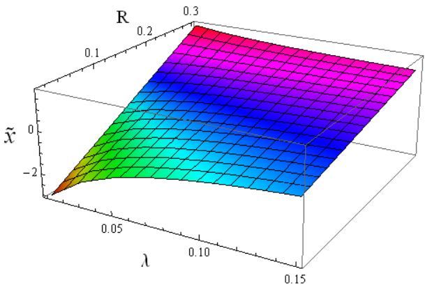
                                 Figure 1 illustrates x̃ against λ and R. Since R is the mininum rate the individual must
                           consume, the wealth threshold x̃ increases with R. An individual with a large force of
                           mortality λ likely tends to consume less than does an individual with a small λ. Therefore,
                           x̃ increases also with λ.

                           Figure 1. The wealth level threshold x̃ against force of mortality and subsistence level of consumption.
                           The parameters: α = 1, β = 0.07, γ = 3, K = 1, y = 0.3, µ = 0.1, σ = 0.2, r = 0.05.

                                 For Figures 2a–4a wealth level threshold x̃1 , x̃2 , and x̃3 stand for x̃ with λ = 0.01,
                           λ = 0.03, and λ = 0.05, respectively. For Figures 2b–4b wealth level threshold x̃1 , x̃2 , and
                           x̃3 stand for x̃ with R = 0.05, R = 0.1, and R = 0.15, respectively.
                                 Figure 2 shows individual’s optimal consumption for various force of mortality λ and
                           subsistence level consumption R. For a given wealth level, an individual with a large force
                           of mortality consume less than does an individual with a small force of mortality. A large
                           force of mortality force an individual reduce consumption. The effect of R on consumption
                           shows the same pattern as that of λ. A strong restriction on minimum consumption level
                           makes an individual to decrease consumption.

                                                  (a)                                                 (b)

                           Figure 2. The parameters: α = 1, β = 0.07, γ = 3, K = 1, y = 0.3, µ = 0.1, σ = 0.2, r = 0.05. (a)
                           Optimal consumption for various force of mortality. R = 0.1. (b) Optimal consumption for various
                           subsistence level of consumption. λ = 0.01.

                                Individual’s preferences for the risky asset for different force of mortality or sub-
                           sistence level of consumption are exhibited in Figure 3. As we can see, a large force of
                           mortality leads an individual to conservative investing. An individual who are more likely
Mathematics 2021, 9, 358                                                                                                    8 of 10

                           to be exposed to the mortality risk may have more demand for hedging the risk so the
                           individual is not unwilling to be exposed the market risk. A large subsistence level of
                           consumption also force an individual to reduce investment in the risky asset. An individual
                           with a strong subsistence consumption constraint is reluctant to take more market risk
                           which may potentially results in lack of the individual’s wealth to meet the subsistence
                           level of consumption.

                                                 (a)                                                  (b)

                           Figure 3. The parameters: α = 1, β = 0.07, γ = 3, K = 1, y = 0.3, µ = 0.1, σ = 0.2, r = 0.05. (a)
                           Optimal portfolio for various force of mortality. R = 0.1. (b) Optimal portfolio for various subsistence
                           level of consumption. λ = 0.01.

                                With a large mortality risk, an individual has a strong demand for life insurance
                           coverage. This is well illustrated in Figure 4a. On the other hand, a large subsistence level
                           of consumption leads to a less demand for life insurance coverage. However, the effect of
                           subsistence level of consumption on life insurance demand is rather marginal, especially
                           for higher wealth levels.

                                                 (a)                                                  (b)

                           Figure 4. The parameters: α = 1, β = 0.07, γ = 3, K = 1, y = 0.3, µ = 0.1, σ = 0.2, r = 0.05. (a)
                           Optimal life insurance for various force of mortality. R = 0.1. (b) Optimal life insurance for various
                           subsistence level of consumption. λ = 0.01.

                                Differently from our study, Ref. [1] employs a CRRA utility to investigate effects of
                           consumption habit on life-contingent claims using term structure of mortality intensity
                           and labor income for considering age effects. The way how the life insurance purchase
                           decision is affected by subsistence consumption (this paper) and consumption habit ([1];
                           the demand for life insurance increases with consumption habit level but also decrease
                           with the level, if the level is very high) are different from each other. Nevertheless, both of
                           the studies reveal that demand for life insurance increases with risk aversion. In Figure 5,
                           we present life insurance purchase against wealth level for diffrent coefficients of absolute
                           risk aversion. A large risk aversion tends to induce more demand for hedging instrument
                           to mitigate income loss due to mortality.
Mathematics 2021, 9, 358                                                                                                           9 of 10

                                  Figure 5. Optimal life insurance for various risk aversion. The parameters: β = 0.07, γ = 3,
                                  R = 0.1, λ = 0.01, K = 1, y = 0.3, µ = 0.1, σ = 0.2, r = 0.05.

                                  6. Conclusions
                                        The purpose this paper is to examine effects of force of mortality and subsistence
                                  level of consumption on an individual’s decision making. With an exponential utility of
                                  consumption while living, we obtain optimal consumption, portfolio, and life insurance
                                  coverage strategies using the martingale and duality method. Numerical illustrations based
                                  on our explicit solution show that a strong force of mortality and a high subsistence level
                                  of consumption lead an individual to reduce exposure to the market risk and to consume
                                  less. An individual with a large mortality risk demands more life insurance coverage as
                                  an individual with a low subsistence level of consumption does. For example, during a
                                  pandemic outbreak, such as COVID-19, the force of mortality increases so the individual
                                  must lessen consumption and have lower risky asset shares, but buy more life insurance.
                                  If successful vaccines are developed, the force of mortality decreases so the individual
                                  consume more, increases long position in the risky asset, and reduce life insurance purchase.
                                  However, our numerical illustrations reveal that the effect of subsistence consumption
                                  constraint on demand for life insurance seems to be marginal. Lastly, we observe that the
                                  demand for life insurance increases with risk aversion.
                                  Funding: This work was supported by the National Research Foundation of Korea Grant funded
                                  by the Korean Government (NRF-2019R1F1A1060853) and by the Research Grant of Kwangwoon
                                  University in 2020.
                                  Institutional Review Board Statement: Not applicable.
                                  Informed Consent Statement: Not applicable.
                                  Data Availability Statement: Not applicable.
                                  Acknowledgments: We highly appreciate the anonymous reviewers for helpful comments and
                                  valuable suggestions.
                                  Conflicts of Interest: The author declares no conflict of interest.

References
1.    Boyle, P.P.; Tan, K.S.; Wei, P.; Zhuang, S.C. Annuity and Insurance Choice Under Habit Formation. Working Paper 2020. Available
      online: https://ssrn.com/abstract=3570066 (accessed on 6 April 2020).
2.    Jang, B.G.; Lee, H.S. Retirement with risk aversion change and borrowing constraints. Financ. Res. Lett. 2016, 16, 112–124.
      [CrossRef]
3.    Jeon, J.; Shin, Y.H. Finite horizon portfolio selection with a negative wealth constraint. J. Comput. Appl. Math. 2019, 15, 329–338.
      [CrossRef]
4.    Koo, J.L.; Ahn, S.R.; Koo, B.L.; Koo, H.K.; Shin, Y.H. Optimal Consumption and Portfolio Selection with Quadratic Utility and a
      Subsistence Consumption Constraint. Stoch. Anal. Appl. 2016, 34, 165–177. [CrossRef]
5.    Kim, J.Y.; Shin, Y.H. Optimal Consumption and Portfolio Selection with Negative Wealth Constraints, Subsistence Consumption
      Constraints, and CARA Utility. J. Korean Stat. Soc. 2018, 47, 509–519. [CrossRef]
6.    Lee. H. Consumption-portfolio choice with subsistence consumption and risk aversion change at retirement. J. Inequalities Appl.
      2018, 2018, 165. [CrossRef] [PubMed]
7.    Lim, B.H.; Kwak, M. Bequest motive and incentive to retire: Consumption, investment, retirement, and life insurance strategies.
      Financ. Res. Lett. 2016, 16, 19–27. [CrossRef]
Mathematics 2021, 9, 358                                                                                                         10 of 10

8.    Lim, B.H.; Lee, H. Household utility maximization with life insurance: A CES utility case. Jpn. J. Ind. Appl. Math. 2020, in press.
      [CrossRef]
9.    Lim, B.H.; Lee, H.; Shin, Y.H. The Effects of Pre-/Post-Retirement Downside Consumption Constraints on Optimal Consumption,
      Portfolio, and Retirement. Financ. Res. Lett. 2018, 25, 213–221. [CrossRef]
10.   Lee, H.; Shin, Y.H. An Optimal Consumption, Investment and Voluntary Retirement Choice Problem with Disutility and
      Subsistence Consumption Constraints: A Dynamic Programming Approach. J. Math. Anal. Appl. 2015, 428, 762–771. [CrossRef]
11.   Lee, H.; Shin, Y.H. An Optimal Investment, Consumption-Leisure and Voluntary Retirement Choice Problem with Subsistence
      Consumption Constraints. Jpn. J. Ind. Appl. Math. 2016, 33, 297–320. [CrossRef]
12.   Lim, B.H.; Shin, Y.H. Optimal Investment, Consumption and Retirement Decision with Disutility and Borrowing Constraints.
      Quant. Financ. 2011, 11, 1581–1592. [CrossRef]
13.   Lim, B.H.; Shin, Y.H.; Choi, U.J. Optimal Investment, Consumption and Retirement Choice Problem with Disutility and
      Subsistence Consumption Constraints. J. Math. Anal. Appl. 2008, 345, 109–122. [CrossRef]
14.   Lee, H.; Shim, G.; Shin, Y.H. Borrowing constraints, effective flexibility in labor supply, and portfolio selection. Math. Financ.
      Econ. 2018, 13, 173–208. [CrossRef]
15.   Park, K.; Kang, M.; Shin, Y.H. An Optimal Consumption, Leisure, and Investment Problem with an Option to Retire and Negative
      Wealth Constraints. Chaos Solitons Fractals 2017, 103, 374–381. [CrossRef]
16.   Park, S.; Jang, B.G. Optimal Retirement Strategy with a Negative Wealth Constraint. Oper. Res. Lett. 2014, 42, 208–212. [CrossRef]
17.   Roh, K.; Kim, J.Y.; Shin, Y.H. An Optimal Consumption and Investment Problem with Quadratic Utility and Negative Wealth
      Constraints. J. Inequalities Appl. 2017, 188, 10. [CrossRef] [PubMed]
18.   Shin, Y.H.; Lim, B.H.; Choi, U.J. Optimal Consumption and Portfolio Selection Problem with Downside Consumption Constraints.
      Appl. Math. Comput. 2007, 188, 1801–1811. [CrossRef]
19.   Shim, G.; Shin, Y.H. Portfolio Selection with Subsistence Consumption Constraints and CARA Utility. Math. Probl. Eng. 2014,
      2014, 153793. [CrossRef]
You can also read