Kullback-Leibler-Based Discrete Relative Risk Models for Integration of Published Prediction Models with New Dataset - arXiv.org
←
→
Page content transcription
If your browser does not render page correctly, please read the page content below
Kullback-Leibler-Based Discrete Relative Risk Models for
                                            Integration of Published Prediction Models with New Dataset

                                                                          Di Wang, Wen Ye, Kevin He
                                                     Department of Biostatistics, University of Michigan, Ann Arbor, MI

                                          Abstract
arXiv:2101.02354v1 [stat.ME] 7 Jan 2021

                                             Existing literature for prediction of time-to-event data has primarily focused on risk
                                          factors from an individual dataset. However, these analyses may suffer from small sample
                                          sizes, high dimensionality and low signal-to-noise ratios. To improve prediction stability and
                                          better understand risk factors associated with outcomes of interest, we propose a Kullback-
                                          Leibler-based discrete relative risk modeling procedure. Simulations and real data analysis
                                          are conducted to show the advantage of the proposed methods compared with those solely
                                          based on local dataset or prior models.

                                          Introduction

                                             Prior research for predicting survival outcomes has primarily focused on risk factors
                                          from an individual dataset. These analyses may suffer from small sample sizes, high di-
                                          mensionality and low signal-to-noise ratios. To address these limitations and improve the
                                          prediction stability, we propose a Kullback-Leibler-based discrete relative risk modeling
                                          procedure to aggregate the new data with previously published prediction models.

                                             Our endeavor is motivated by the prediction of kidney post-transplantation mortality.
                                          With a limited supply of donor kidneys and an increasing need for kidney transplantation,
                                          methods to accurately identify optimal organ allocation are urgently needed. Recently, the
                                          Kidney Donor Profile Index (KDPI) has been introduced to combine a variety of donor
                                          factors into a single number that summarizes the likelihood of graft failure after a deceased
                                          donor kidney transplant. The KDPI has been used to measure how long a deceased donor
                                          kidney is expected to function relative to all of the kidneys recovered in the U.S. Lower
                                          KDPI scores are believed to be associated with longer estimated function, while higher
                                          KDPI scores are associated with shorter estimated function. However, the predictive power

                                                                                        1
of the KDPI is only moderate (C-index = 0.60). In addition, the KDPI does not include
all donor factors potentially associated with kidney graft outcomes. For example, biopsy
results are not included in the KDPI. Since the KDPI is a donor-level measure, not specific
to either kidney, it also does not contain any information about anatomical damage, trauma,
or abnormalities that may be associated with one of a donor’s kidneys. Further, the KDPI
provides no assessment of the likelihood of disease or malignancy transmission from a
deceased donor. Consequently, KDPI is not a precise enough tool to differentiate the
quality of kidney donors.
In addition to the KDPI score, each candidate on the kidney waitlist gets an individual
Estimated Post-Transplant Survival Score (EPTS), ranging from 0 to 100 percent. Can-
didates with EPTS scores of 20 percent or less will receive offers for kidneys from donors
with similar KDPI scores before other candidates at the local, regional, and national levels
of distribution. Similar to KDPI, the predictive power of EPTS is limited. For example,
it has been shown that patients with comorbidities have a greater than 3-fold increase in
event failure risk than patients without comorbidities. The EPTS model, however, does not
make this distinction since comorbidities (except for diabetes mellitus) are not included in
the model.
To optimize the organ allocation and improve our understanding of risk factors asso-
ciated with post-transplant mortality, a desirable strategy is to aggregate these published
survival models with new available dataset. One example for such datasets is the Michigan
Genomics Initiative (MGI), an institutional repository of DNA and genetic data that is
linked to medical phenotype and electronic health record (EHR) information.
In the context of survival analysis, prediction models have primarily focused on individ-
ual dataset. Tibshirani (1997) proposed a Lasso procedure in the Cox proportional hazards
model, and a coordinate descent algorithm for this procedure was developed in the R pack-
age glmnet (Simon et al. 2011). To deal with the problem of collinearity, Simon et al.
(2011) developed the elastic net for the Cox proportional hazards models. Alternatively,
Random Survival Forests (RSF) model (Ishwaran et al. 2008) has been applied for the
2prediction of coronary artery disease mortality (Steele et al. 2018). While successful, these
analyses may suffer from small sample sizes, high dimensionality and low signal-to-noise
ratios. Thus, of special interest in this report is to aggregate the new data with previously
published prediction models, such as the KDPI and EPTS scores for kidney transplanta-
tion. To improve prediction stability and better understand risk factors associated with
outcomes of interest, we propose a Kullback-Leibler-based discrete relative risk modeling
procedure.
Methods
Discrete Relative Risk Models An important consideration for analyses of post-transplant
mortality is that the time is typically recorded on a daily basis. For example, in studies
of 30-day mortality, there are 30 discrete event times and the number of tied events is
numerous. When the number of unique event times reduces, the bias of parameter esti-
mations increases quickly, preventing the use of the standard partial likelihood approach.
These concerns motivate us to propose a prediction approach based on discrete relative risk
models.
Let Ti denote the event time of interest for subject i, i = 1, . . . , n, where n is the total
number of subjects. Let k = 1, . . . , τ be the unique event times (e.g. τ = 30 for 30 day
mortality). Let Dk denote the set of labels associated with individuals failing at time k.
The set of labels associated with individuals censored at time k is denoted as Ck . Let
Rk denote the at risk set at time k. Let Xi be an external and possibly time-dependent
covariate vector for the i-th subject. Let λik = P (Ti = k|Ti ≥ k, Xi ) be the hazard at time
k for the i-th patient with covariate Xi . The likelihood function is given by
τ
( )
Y Y Y
L= (1 − λik ) λik . (1)
k=1 i∈Rk −Dk i∈Dk
Consider a general formulation of the hazard h(λik ) = h(ηk + X>
ik β), where h denotes a
monotonically increasing and twice differentiable link function, ηk is the baseline hazard of
mortality at time k, and β denotes a coefficient vector associated with Xik . Define g = h−1 .
3The log-likelihood is given by
n X τ
g(ηk + X>
ik β)
X
>
`(η, β) = Yik δik log >
+ log{1 − g(ηk + Xik β)} , (2)
i=1 k=1
1 − g(ηk + X ik β)
where Yik is the at-risk indicator and δik is the death indicator at time k. Common
choices for the link function h include complementary log-log (grouped relative risk model),
log (discrete relative risk model), and logit (discrete logistic model).
Kullback-Leibler-Based Integration To integrate the published models, we utilize the
fact that the term
δik log[g(ηk + X> > >
ik β)/{1 − g(ηk + Xik β)}] + log{1 − g(ηk + Xik β)}
in the log-likelihood (2) is proportional to the Kullback–Leibler (KL) distance between the
distribution of the discrete survival model and the corresponding saturated model. The
resulting weighted log-likelihood function to link the prior information and the new data is
given by
n X
τ
" #
g(ηk + X>
X δli + λδ̂ik ik β)
`λ (η, β) = Yik log + log{1 − g(ηk + X>
ik β)} , (3)
i=1 k=1
1+λ 1 − g(ηk + X> ik β)
where δ̂ik = h(η̂k + X>
ik β) is the predicted outcome for subject i at time k based on the
b
risk factors in the new data, and parameters η̂k and βb obtained from the prior model. If
the prior model only contains a subset of relevant variables in the new data, the remaining
values of βb are set to be 0. Note that λ is a tuning parameter to weigh the prior information
and the new data and is determined using cross-validation. In the extreme case of λ = 0,
the penalized log-likelihood is reduced to the log-likelihood based on the new data. In
contrast, when λ = ∞, the model is equivalent to the prior information.
Simulation
To assess the performance of the proposed procedure, we compared it with both the
prior model and the model fitted only by local data. Generally, the proposed KL modeling
procedure works for log-log, log and logit link functions. Here, we used logit link as an
4example function to conduct the simulation studies. Suppose β0 = (β0 , β1 , . . . , βp0 )T is
the vector of coefficients from a prior model published in the previous research, and βl =
(β0 , β1 , . . . , βpn )T is the vector of coefficients from which the local data is generated. We
assume that the prior model and the local data share the same set of baseline hazard of
mortality ηk at each discrete time point Tk . Then the local training data is generated by
X ∼ M V N (0, Σ), where Σ is a first-order autoregressive (AR1) correlation matrix with
the auto-correlation parameter 0.5. For each time point Tk , the event indicator Yik for each
subject i in the at risk set Rk is generated by Bernoulli(logit−1 (XiT βl + ηk )). We will delete
subject i from the at risk set RT >Tk for future time points if Yik = 1 at Tk ; otherwise, we
will keep it. Latent censoring times are generated from a discrete uniform(1, 30), and then
are truncated by an administrative censoring at time point 10.
We consider six different models which are clustered into two scenarios in the simulation
studies:
Scenario 1: Local data and prior model share the same set of predictors:
Model (a): βl = β0 ;
Model (b): βl = 0.5β0 ;
Model (c): βl =reverse(β0 ) = (βp0 , βp0 −1 , . . . , β0 )T .
Scenario 2: Local data contains all predictors in the prior model and additional new
predictors:
Model (d): βl = (β0 , 0.2β0 );
Model (e): βl = (β0 , 0.5β0 );
Model (f): βl = (β0 , β0 ).
For scenario 1, model (a) mimics the situation when local data comes from exactly the
same model as the prior model; model (b) changes the magnitude of coefficients from the
prior model, but keeps the same trend; the local data in model (c) is generated from a
completely different model. For scenario 2, model (d), (e) and (f) mimic the situations
where the additional new predictors in the local data are of various importance compared
5to the prior model, which are managed by adjusting magnitudes of the new predictors.
Moreover, we set the local sample size nl = 300, number of prior predictors p0 = 10,
number of additional new predictors pn = 10 and the range of tuning parameters to be
λ ∈ [0, 10].
The tuning parameter λ is selected by 5-fold cross validation on the local data with
empirical log likelihood as the metric of model performance. After determining λ, we
evaluate the proposed KL modeling method with the prior model and the local model. In
order to make a fair comparison, we evaluate the models on the hold-out external validation
data set, which is simulated from the same model setting as the local data. The best model
achieves the maximal log likelihood on the external validation dataset. The simulation is
replicated 100 times.
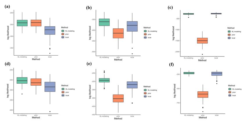
Figure 1: Simulation results of KL-modeling (green) compared with prior (red) and local
(purple) models. (a)-(f) presents results for model setting (a)-(f) respectively.
Figure 1 shows that under all model settings the KL-based modeling procedure achieves
comparable or better performance than both the prior model and the model fitted only
by the local data. More specifically, the KL-based modeling procedure favors the cases
where the prior model is similar to the local data. However, even under extreme situations
when the prior model is completely different from the local data (Fig. 1 (c)) or missing
important predictors (Fig. 1 (f)), the KL-based modeling procedure does not result in
misleading predictions. We also present the best tuning parameter λ determined by the
6KL-based modeling procedure in the simulation studies. The KL-based modeling procedure
tends to select larger λ when the prior model is more similar to the local data. In addition,
it will not incorporate bad prior information which is not relevant to the local data by
selecting an extremely small λ or setting it to be 0 (Figure 2).
Figure 2: Selected tuning parameter λ for the best fitting of KL modeling procedure. (a)-(f)
represents model setting (a)-(f) respectively.
Data Analysis
We use EPTS model and a local kidney transplant data as an example to illustrate
how to use KL modeling procedure to integrate previously published prediction models
and new dataset. The raw EPTS score is derived from a Cox proportional hazards model
using Scientific Registry of Transplant Recipients (SRTR) kidney transplant data. For sim-
plicity, the raw EPTS score only includes 4 predictors in the model: candidate’s age in
years, duration on dialysis in years, current diagnosis of diabetes, and whether the candi-
date has a prior organ transplant. Since the EPTS model doesn’t report baseline survival
information, we applied estimated baseline survival information using kidney transplant
data obtained from the U.S. Organ Procurement and Transplantation Network (OPTN)
(https://optn.transplant.hrsa.gov/data/). A total of 80,019 patients which includes all pa-
tients with ages greater than 18 who received transplant between January 2005 and January
7Scenario 1
Model KL Prior Local
log likelihood -358.478 -398.657 -395.531
Scenario 2
Model KL Prior Local
log likelihood -358.467 -398.657 -409.814
Table 1: The log likelihood of different models.
2013 with deceased donor type were used in the estimation. Specifically, we fit a discrete
relative risk model including the same set of predictors as EPTS model does and obtained
the parameter estimates for each week within the first year after receiving transplants.
Thus, our prior model is the combination of EPTS model and estimated baseline survival
information by week.
The local kidney transplant data we used is the University of Michigan Medical Center
(MIUM) kidney transplant dataset. We consider two different scenarios regarding to predic-
tors of local data: Scenario 1, which includes the same set of predictors as EPTS does, and
Scenario 2, which includes two additional predictors of comorbidities (whether candidate
has previous malignancy, and presence of pre-transplant peripheral vascular disease) than
EPTS. In this real data analysis, we only evaluate first year survival after transplant. As
shown in Table 1, KL-based modeling procedure has the best performance under both two
scenarios. Specifically, using the same set of predictors, the model fitted only by local data
has a slightly better performance than prior model, which indicates that the prior model
lacks accuracy when applied to this specific local dataset. However, the log likelihood of
the local model decreases substantially when including additional predictors, which shows
that the model fitted only by local dataset is unstable. In summary, KL-based modeling
procedure provides a more stable and accurate prediction than the prior model and the
model fitted only by the local data.
8Summary
Existing literature for prediction of time-to-event data has primarily focused on risk
factors from an individual dataset, which may suffer from small sample sizes, high dimen-
sionality and low signal-to-noise ratios. To improve prediction stability and better under-
stand risk factors associated with outcomes of interest, we propose a Kullback-Leibler-based
discrete relative risk modeling procedure. Simulations are conducted to show the advan-
tage of the proposed methods compared with those solely based on local dataset or prior
models. The proposed Kullback-Leibler-based discrete relative risk modeling procedure is
sufficiently flexible to incorporate situations where the number of risk factors in the MGI
dataset is greater than those available in previous models reported in the literature.
References
Kalbfleisch, J.D., and Prentice, R.L. 1973. Marginal likelihoods based on Cox’s regression
and life model. Biometrika 60(2): 267–278.
Simon, N.; Friedman, J.; Hastie, T.; and Tibshirani, R. 2011. Regularization Paths for
Cox’s Proportional Hazards Model via Coordinate Descent. Journal of statistical software
39(5): 1–13.
Ishwaran, H.; Kogalur, U.B.; Blackstone, E.H.; and Lauer, M.S. 2008. Random survival
forests. The annals of applied statistics 2(3): 841–860.
Steele, A.J.; Denaxas, S.C.; Shah, A.D.; Hemingway, H.; and Luscombe, N.M. 2018.
Machine learning models in electronic health records can outperform conventional sur-
vival models for predicting patient mortality in coronary artery disease. PloS one 13(8):
e0202344.
9You can also read