Living wages and age discontinuities for low-wage workers - Discussion Paper

Discussion Paper ISSN 2042-2695

No.1803
September 2021

Living wages and
age discontinuities
for low-wage
workers

Nikhil Datta
Stephen Machin

Abstract
This paper considers an emerging, highly policy relevant feature of minimum wages, studying what happens
when a wage floor significantly higher than a nationally legislated minimum is imposed. The consequences
of age-wage discontinuities and wage floors higher than mandated minimum wages are explored in the
context of a Living Wage being introduced to a large UK organisation through time. Between 2011 and
2019, the Company was exposed to a Living Wage Rate higher than the statutory National Minimum Wage,
which was sequentially introduced into some of its establishments and had the effect of boosting wages and
strongly increasing the age-wage discontinuity from age-related pay grades. The analysis finds positive
labour supply responses at the age discontinuity before Living Wage treatment, but a fall in hours at the
discontinuity following treatment. The Living Wage raised wage costs but did not affect aggregate hours,
showing a within-establishment reallocation of hours by age arising from differential eligibility to be paid
the Living Wage.

Key words: living wages, minimum wages, wages, hours
JEL: J31; J38; J42

This paper was produced as part of the Centre’s Labour Markets Programme. The Centre for Economic
Performance is financed by the Economic and Social Research Council.

This research was funded by the Economic and Social Research Council at the Centre for Economic
Performance and the UBEL Doctoral Training Partnership. We additionally thank The Living Wage
Foundation for institutional information regarding the Living Wage, and The Company for use of the data.
 Nikhil Datta, University College London and Centre for Economic Performance, London School of
Economics. Stephen Machin, Department of Economics and Centre for Economic Performance, London
School of Economics.

Published by
Centre for Economic Performance
London School of Economics and Political Science
Houghton Street
London WC2A 2AE

All rights reserved. No part of this publication may be reproduced, stored in a retrieval system or transmitted
in any form or by any means without the prior permission in writing of the publisher nor be issued to the
public or circulated in any form other than that in which it is published.

Requests for permission to reproduce any article or part of the Working Paper should be sent to the editor at
the above address.

 N. Datta and S. Machin, submitted 2021.

1. Introduction

 Study of minimum wages, and their economic effects, has once again become a common

preoccupation of researchers. There are a number of reasons why. Many countries are

experiencing low real wage growth and a minimum wage policy is one that can directly boost

the wages of low wage workers. Viewed through this lens, minimum wages have become the

policy tool of choice as some places – like US and UK cities – have decided to raise local

minimum wages above the presiding national or state legislated minimum wage. Some

companies (for example, Amazon, IKEA, Wal-Mart) have raised their own lowest wage above

the mandated minimum. And in the recent past some countries, most notably Germany in 2015,

that did not previously have a national minimum wage have introduced one at a relatively high

level.

 These features of minimum wages have resulted in a sizable upsurge of recent research

which has broadened the remit in this area. A clear focus has been placed on studying newer

questions relative to the very sizeable past research literature that placed a principal focus on

studying the employment effects of minimum wages.1 Because of the widespread finding from

a range of studies that the employment effects tend to be modest, if they exist at all, more recent

research looks at other forms of adjustment to the wage cost shock that minimum wages induce

(see, for example, Draca, Machin and Van Reenen, 2011, Hirsch, Kaufman and Zelenska, 2015,

Bell and Machin, 2018, and Harasztori and Linder, 2019), on changes in the composition of

worker wages and employment (Giuliano, 2013, Dustmann, Lindner, Schönberg, Umkehrer

1
 The various phases of minimum wage research are summarised well in reviews by Brown, Gilroy and Kohen
(1982) on the first generation of time series studies, by Card and Krueger (2004) on the second generation of so-
called “revisionist” quasi-experimental research and by Brown (1999) on both. See also a review making closer
links between minimum wage research and monopsony in the labour market by Manning (2021).
 1

and Von Berge, 2020, and Giupponi and Machin, 2021) and on local minimum wages (Dube

and Lindner, 2021).

 This paper studies an emerging, highly policy relevant feature of minimum wages. It

studies what happens when a significantly higher wage floor than a nationally legislated

minimum is imposed. It is able to adopt a research design where some establishments of a firm

progressively raised their minimum wage floor to a level higher than the prevailing national

minimum wage. The setting is the UK, where the company studied was exposed to a Living

Wage Rate higher than the statutory National Minimum Wage sequentially as it was introduced

into some of its establishments in a staggered sequence between 2012 and 2019. The Company

is an employer of a large number of low wage workers with over 300 establishments across the

UK and operates in the service sector. While the Company’s main competitors are firms

operating in the private sector, a large part of the firm’s business is government procurement

contracts.

 A new focus has emerged in recent years on living wages, wage rates which are required

to meet minimum standards given the costs of living. In the UK this is exemplified by the

Living Wage Foundation which calculates rates for London and the rest of the UK and has

accredited over 7,000 employers. In the US MIT operate a living wage calculator for different

states, cities and metro areas (Glasmeier, 2020) and hundreds of cities have passed living-wage

ordinances (Dube and Lindner, 2021; Sosnaud, 2016).2 This interest has emerged at least in

part as a result of claims that national minimum wage levels (or federal and state minima in the

US) have not been adequate to meet the cost of living (Iacurci, 2021). This paper presents a

2
 Many of these US city living wage ordinances are lower than the rate as recommended by the MIT Living Wage
Calculator for the area and are more precisely de facto higher local minimum wages, not living wages.
 2

detailed account of how firms respond to a “true” living wage, calculated according to a

consumption basket of goods and services deemed necessary for an acceptable standard of

living.3

 The paper studies the impact of introducing the Living Wage Rate on wages and hours in

The Company, leveraging two sources of credibly exogenous variation: a staggered mandated

Living Wage treatment and a discontinuity in the age-wage profile. Due to age eligibility

criteria for the Living Wage the interaction of these two effects results in differential

discontinuities in the age-wage profile for treated and untreated establishments. Thus, the

setting lends itself to an event study research design, a regression discontinuity design, and the

interaction of these two which is referred to as a “difference-in-discontinuity” design. The

analysis finds that the Living Wage raised wages but did not damage aggregate jobs and hours.

It did, however, result in a reallocation of workers by age because of differential eligibility to

be paid the Living Wage. In particular we find that younger workers around the age eligibility

cut-off experience a loss of hours and, in some cases, earnings as the firm is able to substitute

them with older workers, as a direct result of the Living Wage introduction.

2. The Experimental Setting

 The Living Wage Foundation (LWF) is a charitable organisation in the UK, established

in 2011, that campaigns for employers to pay workers a living wage. Each year the LWF

calculates and publishes a Living Wage rate for London (LLW) and the rest of the UK

(UKLW). The LLW rate has typically been approximately 30-35% higher than the official

3
 For details of the methodology underpinning the calculation, and the history of the UK Living Wage, see D’Arcy
and Finch (2019).
 3

statutory National Minimum Wage (NMW) applicable to over 21s, or National Living Wage

(NLW) applicable to over 25s, while the UKLW has been about 15-20% higher as can be seen

in Figure A1 of the Appendix. However, unlike the statutory NMW, the LLW and UKLW

comprise only of a single rate which is applicable to all workers over the age of 18, with 16

and 17 year olds in work not being covered by the Living Wage. The NMW on the other hand

is currently comprised of 4 different age-specific rates: age 16-17, age 18–20, age 21-24 and

age 25+.

 Organisations voluntarily sign up to become Living Wage employers and following

appropriate audits by the LWF can achieve accredited status. As of July 2020, the LWF lists

6,562 accredited employers and included in this list are 107 local government units.4 When

public bodies achieve accreditation, they are given an amnesty on existing procurement

contracts, but are expected to enforce the living wage at the start, renegotiation or renewal of

contracts.

 The Company operates in the service sector and the majority of their business is through

procurement contracts with local councils.5 As the firm operates hundreds of establishments

across the UK, different establishments become contractually obliged to pay the LLW and

UKLW at different times. This is dependent on whether, and when, the local government unit

has voluntarily signed up to the LWF’s Living Wage, as well as idiosyncratic timings of

contractual renewal or renegotiation.

4
 These include London Boroughs, Unitary Authorities, Metropolitan Districts, County Councils, District
Councils, Local Government Districts and Parish Councils.
5
 Councils here refer to Principal Councils which are local government authorities carrying out statutory duties in
England and Wales. They are responsible for a wide range of public services including transport, education,
planning, and cultural services, and operate local tax collection. There are 355 principal councils in England and
Wales and this includes 33 London boroughs.
 4

Between 2012 and 2019, 107 local government units gained accreditation. For example,

of the 32 London Boroughs, 17 have received accreditation, the earliest (Islington in North

London) receiving accreditation in May 2012, and the most recent (Redbridge in the East of

the city) receiving accreditation in November 2018.6 As Exhibit 1 shows, this setting gives

substantial variation in Living Wage treatment for establishments run by The Company. In

particular, over the period for which we have HR data approximately 140 establishments went

from being untreated to treated, while run by The Company. The remainder never pay Living

Wages and the relevant minimum wage floor to them is the UK National Minimum Wage.

 This variation in Living Wage treatment is combined with the fact that The Company

has an already existent pay structure which operates an age-related pay scale for their entry-

level (unskilled) jobs.7 In particular, similar to the NMW, their pay-scale has a sizeable

discontinuity at age 18.8 The Living Wage treatment, which only treats those over 18, therefore

has the effect of increasing the size of this age-wage discontinuity. It is thus possible to

implement a “Differences-in-Discontinuity” design, exploiting both an exogenous treatment to

wages as well as a seemingly arbitrary discontinuity in wages as a function of age, where the

treatment effects the size of the discontinuity.

 The setting combined with the dataset allows a novel analysis of how a wage floor could

affect highly exposed young workers employed on casual contracts (specifically on zero-hours

contracts9), both in terms of wages and employment along the intensive margin. The presence

6
 Correct as of July 2019.
7
 This pay-scale is centrally determined, however establishments have independent control over both intensive
and extensive margin employment, as well as employment composition.
8
 Many companies have a sizeable discontinuity at this particular age, when individuals become adults in UK
law. The NMW for example as of April 2020 implies a statutory rate of £4.55 for under 18s and a statutory rate
of £6.45 for age 18-20.
9
 For a complete description of the of what these types of contracts entail see Datta, Giupponi and Machin (2019).
 5

of the discontinuity at age 18 would likely result in both supply and demand effects, where

young workers would be willing to supply more labour just after the age 18 cut-off, and budget

conscious managers would be less willing to give such workers as many hours. Furthermore,

when an establishment is exposed to a higher wage floor it is likely that labour supply to the

establishment across the whole age range would increase, potentially suppressing demand for

younger workers.10 By comparing the size of the discontinuity in wages and hours before and

after treatment, the analysis is able to disentangle which of these effects dominates, and thus

assess the impact on young workers.

 As all establishments are operated by the same company using the same structure of

operations and management, but with establishment level autonomy over employment and

workforce composition, a true counterfactual, when comparing treated and untreated

establishments, can be estimated. Additionally, unlike in many minimum wage papers, the

approach can isolate the impact of just the individual establishment being exposed to a higher

wage floor, rather than the entire market. This is because when a local government unit

voluntarily signs up to the LWF’s Living Wage, private companies and non-council public

employees in the area remain untreated.11 Furthermore, the establishment located within the

treated council would not be contractually obliged to the Living Wage until renewal or

renegotiation, introducing further idiosyncrasies in when the establishment must raise wages.

Thus, estimates are not likely to be contaminated by general equilibrium effects.

10
 See Datta (2021) for evidence of this.
11
 The proportion of workers treated within a local authority is a small fraction of a percentage. Council
employment only makes up approximately 3% of employment and typical council jobs are paid above the wage
floor. For more information see Datta (2021).
 6

3. Data and Empirical Method

Data

 This study analyses a novel dataset which contains the complete HR data of The

Company for the period of 2011–2019. As stated in the introduction, The Company operates

in the service sector and a large portion of its turnover is from government procurement

contracts, for local council services. It is worth noting that the council services they provide

are not typical natural monopolies, and other private firms compete in the same local markets.

 The HR data contains very detailed information on all workers in each of The

Company’s establishments. In addition to the usual information such as job tenure, wages, age

and demographic characteristics, there is very detailed data on the specific job role that each

worker carries out, the precise dates of wage changes, and exact hours worked from timesheet

data.

 Table A1 in the Appendix presents summary statistics for workers employed by The

Company as of 2019. The Company is big, employing approximately 19,000 workers and has

a large proportion of female workers (60%). Half of the workers are based in London and 5%

of all workers are less than 18 years old, this proportion is considerably higher for casual entry-

level workers (12%). The workforce is younger on average (36 years) than the national average

(43 years), and this is more pronounced at 31 years old for entry-level workers. Three quarters

of entry-level workers are on casual contracts which puts The Company in a very flexible

position to adjust employment along the intensive margin.

 The average hourly wage is £12.88 per hour, which is approximately 25% lower than

the average hourly wage for the UK in 2019.12 The average hourly wage for entry-level workers

12
 This stood at £17.27, as calculated from the Annual Survey of Hours and Earnings.
 7

is £9.38, almost half of the UK mean and about 15% higher than the UK National Living Wage

shown in Appendix Figure A1. The average worker works approximately only one quarter of

full-time hours, casual entry-level workers only work on average about 5 hours per week.

Given the large proportion of casual staff the summary statistics suggest that permanent

employees work much closer to full time hours (the exact figure is 132 hours per month for the

mean permanent employee). This is in line with the national average.13

Empirical Method 1 – Differences-in-Discontinuity

 The first part of the empirical analysis leverages a “Differences-in-Discontinuity”

research design, to estimate the effect of the key variables – the Living Wage, the age

discontinuity at age 18 and the interaction of the two - on the wages and hours of entry-level

casual workers. Age is normalised around 18 such that = ∗ − 18, where ∗ is the

true measure of age, the discontinuity ( ) is defined = [ ≥ 0], and treatment from

Living Wage introduction (T = 1 when introduced), the wage equation for entry-level casual

worker i employed at establishment e in year y and month m takes the form:

 ( ) = + + + 
 + + (1)
 + + + + 

 This equation has the same format as a typical regression discontinuity design with a linear

predictor for the running variable (age in months above/below 18) either side of the

discontinuity. In addition, however, the specification allows for the pre 18 and post 18 slopes

to differ based on whether the Living Wage treatment has been applied. Additionally, equation

(1) includes both establishment (γ) and year-month fixed effects (λ), as is conventional in a

difference-in-difference specification.

13
 140 hours per week, as calculated from the Annual Survey of Hours and Earnings.
 8

The main parameters of interest are and . In the specification, identifies the impact

of the age discontinuity in the pay-scale schedule on wages, while identifies the impact of

the Living Wage treatment on the size of this wage discontinuity. If the Living Wage raises

wage levels and generates an additional premium for reaching age 18, is expected to be

positive and this is the first key hypothesis to be tested in the analysis.

 After the first stage wage equation, the analysis then considers whether there is an

intensive margin employment response to Living Wage introduction. This first stage of wages

and second stage of labour adjustment, of course, is predicated on the same logical basis as the

way the big literature on minimum wages and employment proceeds, except here we are

looking at a wage floor higher than the mandated minimum. To investigate this second stage,

the same structure specification (1) is adopted, except now with hours worked as the dependent

variable:

 ln (ℎ ) = + + + 
 + + (2)
 + + + + 

 Now the two main parameters of interest are and . In (2), identifies the impact of

the age discontinuity in the pay-scale schedule on hours, while identifies the impact of the

Living Wage treatment on the size of the hours discontinuity. Equation (1) and equation (2) are

estimated on both a wide window of 24 months either side of the age cut-off (i.e. on the sample

of 16 to 20 year olds), and a smaller window of 12 months either side of the age cut-off (i.e.

for 17 to 19 year olds).

 As discussed in section 2, the impact of the increase on wages on hours worked is ex ante

ambiguous. This is because an increase in wages should in theory have oppositely signed labour
 9

supply and demand responses. In the case of > 0, this would suggest the labour supply

response of the age-wage discontinuity dominating the labour demand response, and vice versa.

Similarly, < 0 would suggest that the Living Wage is resulting in some intensive margin

unemployment effects for those workers around the age 18 discontinuity. Furthermore,

depending on the sign of , it is possible to place lower bounds on the labour supply elasticity,

by dividing the respective parameter by its counterpart parameter from specification (1). For

example, if > 0, then gives a lower bound on the labour supply elasticity for casual youth

workers. This is because the labour demand response can be reasonably assumed to be weakly

negative and would contain both supply and demand effects.

Empirical Method 2 – Event Study

 The approach in Empirical Method 1 is informative for generating evidence about local

impacts around the age 18 cut-off, thereby precisely showing how the Company is able to

adjust to the LW introductions. To study how this local adjustment translates into an impact

for the establishment as a whole, and therefore to ascertain whether the Living Wage has an

impact on aggregate wages, employment and hours on the intensive margin, an event study

estimator is implemented at the establishment level which treats the multiple treatment timing

of the setting with due caution.

 Borrowing notation from Sun and Abraham (2020), let denote an outcome of interest

for establishment at year-month ym with treatment status ∈ {0,1}: = 1 if is

treated in period ym and = 0 otherwise, where treatment is absorbing, and therefore

 ≤ for < . An establishment’s treatment path can therefore be characterised by

 = { : = 1}, and = ∞ if the establishment is never treated. Establishments

 10

can therefore be categorized into disjoint cohorts ∈ { , … . , , ∞}, where

establishments in cohort are first treated at the same time { : = }. is the potential

outcome in period ym when establishment is first treated at time and is the potential

outcome at time ym if establishment e never receives treatment. A cohort-specific average

treatment effect on the treated periods from treatment is thus:

 , = , − , = ] (3)

This notation allows for treatment effect heterogeneity across cohorts, which in this setting

may be important as the bite of the living wage may change over time. The key estimate of

interest is then some weighted average of (3), for ∈ , to construct a relative period

coefficient. As is often the case when firms face a shock to the wage floor, the interest is in the

average dynamic effects (which allows an analysis of the pre-trends).

 For analysing these average dynamic effects, a weighted average similar to that proposed

in Sun and Abraham (2020) is

 1 (4)
 = , { = | ∈ }
 | |
 ∈

which effectively uses weights according to the size of the treated cohort that experiences 

periods relative to treatment. In practice, (4) is estimated using the following methodology:

 1. For each treatment cohort estimate an adjusted form of the typical, two-way fixed effect

 event study specification, limiting to 12 months before and after the treatment period.

 = + + , , + ′ + (5)
 ,

 where variables are the same as above, and is a set of time varying establishment

 level controls. For each treatment cohort , the control group is restricted such that
 11

they have not received treatment within the past two years or will not receive treatment

 within two years of the relevant treatment cohort treatment date. This is to ensure no

 overlap of dynamic effects between the treated and control groups. As per the

 suggestion of Borusyak and Jaravel (2017), the dynamic effects are normalised to two

 periods, -1 and -12, to deal with the underidentification issues they raise.

 2. Estimate the weights { = | ∈ } by sample shares of each cohort in the

 relevant relative period .

 3. Combine steps 1 and 2, and aggregate monthly affects , to the level of quarters, ,

 for graphical representation by taking a simple equal weighted mean. In particular

 1 (6)
 ^ = ^ , 
 ^ { = | ∈ }
 3
 ∈

 There has been a recent surge in interest in the workings of difference-in-difference and

event study estimators, especially when there is variation in treatment timing and heterogenous

treatment effects (for example, see Callaway and Sant’Anna, 2021; Goodman-Bacon, 2021;

Sun and Abraham, 2020; and Borusyak and Jaravel, 2017). Concerns raised include: issues

identifying the linear component of the path of pre-trends in traditional event study

specifications (Borusyak and Jaravel, 2017), contamination of lead and lag coefficients from

other period effects (Sun and Abraham, 2020), biased estimates of treatment effects when the

control group contains treated units when dynamic treatment effects are present (Goodman-

Bacon, 2021) and the structure of weights assigned across treatment cohorts when estimating

dynamic treatment effects (Sun and Abraham, 2020). The estimator used here is akin to that

 12

suggested in Sun and Abraham (2020) and also implements adjustment as recommended in

Borusyak and Jaravel (2017) in an attempt to overcome the aforementioned issues.14

Empirical Method - Robustness

 The approach used in the main estimating equations (1) and (2) is more flexible than the

standard two-way fixed effect estimator used in a typical difference-in-difference setting as it

exploits variation in both Living Wage treatment and the discontinuity at age 18. Despite this,

as a matter of caution we additionally implement a robustness check where we compare the

Living Wage impacts on wages from the event study estimates using the Sun and Abraham

(2020) style estimator with a traditional event study regression of the form:

 ln ( ) = + + , + ′ + (7)
 ,

aggregated to quarterly effects according to

 1 (8)
 ^ = ^ .
 3
 ∈

Assuming the estimates of ^ from equation (8) are similar to those from equation (6), which

is robust to the aforementioned issues, this is suggestive that the main estimating equations (1)

and (2) are unlikely to suffer from the above issues.

4. Results

 This section presents the findings, beginning with the first and second stage wage and

hours differences-in-discontinuity-based estimates, moving to consider aggregate

establishment level impacts, and then offering an interpretation of the key results.

14
 For a more complete discussion of some of the discussed issues and how the implemented event study
estimator deals with these, see Datta and Machin (2021).
 13

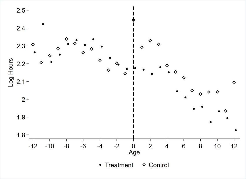
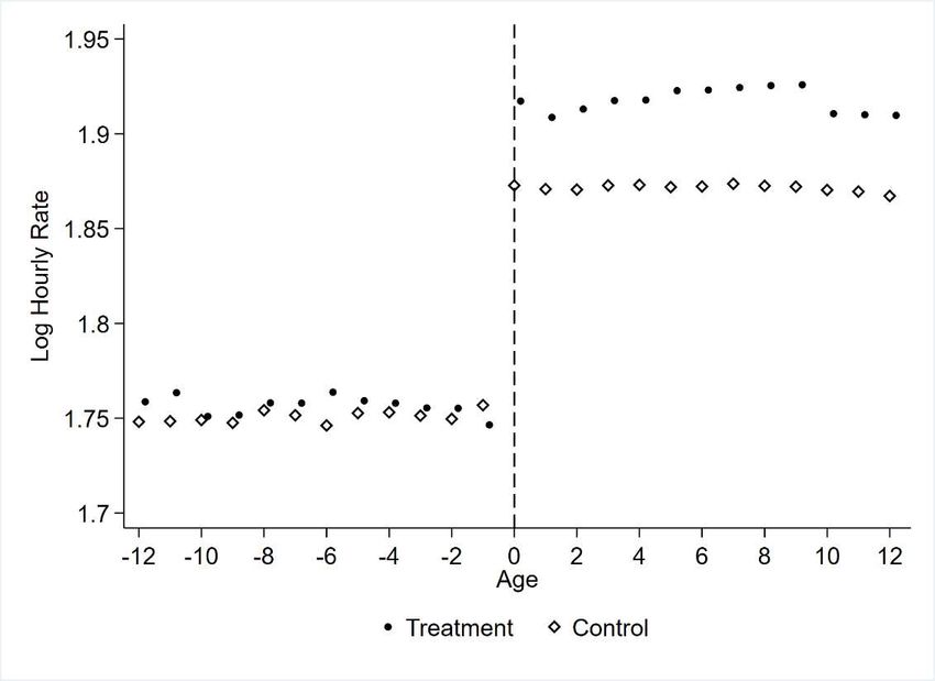
Wages

 Exhibit 2(a) reports scatter plots of the mean log wage by months relative to age 18 for

entry-level casual workers in establishments treated and untreated with the Living Wage,

orthogonalized against time and year fixed effects. There is a clear discontinuity at age 18 in

both cases, and either side of the discontinuity the wage to age correlation appears mostly flat.

The size of the discontinuity for workers in treated centres (approximately 18 log points) is

considerably larger than the discontinuity in untreated centres (approximately 12 log points).

 Columns (1) and (2) of Exhibit 3 present results from the counterpart regressions to

Exhibit 2(a), from estimating specification (1). The parameter estimates suggest in untreated

establishments as an entry-level casual worker moves from age 17 to 18 they experience a 12%

increase in wages. For those in treated establishments the increase in wages is considerably

higher, at about 20%. Workers within the sample also experience on average 4-5% higher

wages from Living Wage treatment. This figure is likely to be higher when considering all

entry-level workers rather than those just around the age 18 cut-off, given the proportion

receiving direct treatment would be larger. The estimates of the main parameters of interest for

specification (1) do not fundamentally vary based on the width of the window considered

around the age 18 cut-off and all are highly statistically significant.

Hours

 Exhibit 2(b) is of the exact same form as Exhibit 2(a) for wages, but instead shows mean

log hours by months relative to age 18. Unsurprisingly, the number of log hours worked

features more noise than its wage counterpart. But the figure shows a positive discontinuity in

log hours at age 18 for workers untreated with the Living Wage, and a structural difference in

this discontinuity for those treated with the Living Wage.

 14

Columns 3 and 4 of Exhibit 4 reports parameter estimates for specification (2) to confirm

this. In particular, the estimates show that as casual entry-level workers move from age 17 to

18, they work 10-17% more hours. The positive sign and size of this parameter suggests a

strong labour supply response from casual youth workers. In the presence of no demand effects,

this would imply a labour supply elasticity of approximately 1.3 according to the specification

using the smaller window.15

 For those in treated establishments, the discontinuity in casual hours drops between 26-

33 percentage points, indicative that the change in hours around the discontinuity becomes

negative. According to the specification using the ±12 month window, hours fall for workers

as they move to the positive side of the discontinuity by approximately 10% in treated

establishments. Both columns 3 and 4 therefore reveal a strong negative impact on intensive

margin employment for casual youth workers just over the age 18 cut-off as a result of a higher

wage floor. Parameter estimates for and imply that casual youth workers around the age

18 cut-off experience a 7% increase in wages due to the Living Wage treatment, but a fall in

hours of 26-33%.16

Aggregate Effects

 Exhibit 4 graphically reports the coefficients from (6) and examines the aggregate effects

at the establishment level of the Living Wage on intensive margin employment. Column (1) in

Table A2 in the appendix presents the counterpart point estimates and standard errors. As can

15
 The elasticity when using the wider window is 0.8 which, even if a little smaller in magnitude, still very
clearly supports the interpretation of a strong supply side response to the Living Wage.
16
 Spatial heterogeneity analysis suggests that workers around the age 18 cut-off in London experienced a 10.3%
increase in wages due to the Living Wage treatment (standard error 0.027), and a fall in hours of 36.5% (standard
error 0.131). The parameter estimates of (0.098, standard error 0.007)) and (0.126, standard error 0.068) for
the 12-month window for those in London suggest a lower bound labour supply elasticity of 1.3, identical to the
main specification.
 15

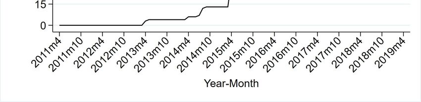
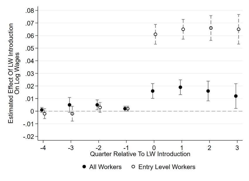
be seen there is an absence of differing pre-trends suggesting that the common time trend

assumption necessary in such settings is not violated. Following the Living Wage introduction

there is no change in aggregate intensive margin employment.17 Figures A2 and A3 in the

Appendix, present event study figures for log wages using parameter estimates from equations

(6) (the robust estimator) and (8) (the traditional estimator) respectively. Columns (2)-(5) in

Table A2 in the appendix present the counterpart point estimates and standard errors. The

figures show a sharp, statistically significant rise in wages for all workers (approximately 1.5%)

and entry-level workers (approximately 6.5%) which is roughly consistent throughout the year

following treatment. The results between the two estimators are strikingly similar which

suggests our main estimating equations are unlikely to be biased by the issues mentioned in

section 3.

 These results suggest that the Living Wage introduction acted to affect the way that hours

are distributed across workers within the establishment, but not the total number of hours

worked. In particular, hours are shifted away from casual workers who have just crossed the

age 18 boundary where the Living Wage becomes binding. Those in treated centres crossing

the boundary experience a 19% increase in wages, and a drop in hours of 10-22% depending

on specification, suggesting the impact on earnings could be negative. Against the

counterfactual of those in untreated centres, who experience a 12% increase in wages and an

increase in hours of 10-16% the fall in earnings is even more pronounced.

Discussion

 The above results can be rationalised and explained in a simple model of a firm with

monopsony power in the labour market. This is illustrated in Exhibit 5. The coefficients on 

17
 Impacts on aggregate employment are reported in Datta and Machin (2021) and similarly show no effects.
 16

and imply a lower bound on the labour supply elasticity to the firm for 18 year olds of

approximately 1.3. This is represented on the diagram by the movement from E

This paper offers novel evidence on how firms respond to a living wage, specifically the

Living Wage Foundation’s Living Wage, which is considerably higher than the UK mandated

minimum wage. Using a bespoke dataset for a large service sector firm with hundreds of

establishments across the UK that are as good as randomly exposed to a Living Wage, this

paper shows that the Living Wage had a strong impact on wages and no aggregate impact on

total hours worked. However, utilising discontinuities in the age-wage profile for The

Company which change in size as a result of exposure to the Living Wage, the analysis

demonstrates that exposed establishments reallocate hours away from workers just over the age

18 cut-off. Because of this hours reallocation, the results suggest that workers just over the age

18 cut-off actually experience a loss of earnings as a result of the living wage introduction, and

establishments are able to do this due to increased labour supply from older, possibly more

productive, workers.

 The results in this paper should be interpreted carefully, at least partly because they apply

to a single firm. In a setting where all (or more) firms are exposed to a higher minimum wage

it is not clear that firms would be able to reallocate hours in the same way, as labour supply

responses would likely be muted. Likewise, for an industry specific Living Wage, for example

the case of social care referred to above, the extent of hours reallocation will depend on the

labour supply elasticity to the market rather than the firm, which is also likely to be

considerably smaller. The main finding of the paper does, however, suggest that there are

settings where firms can absorb higher wage costs in adjustment to a living wage level higher

than the prevailing mandated minimum wage, and in the one studied here this seems largely

due to the presence of monopsony power.

 18

References

Bell, Brian and Stephen Machin (2018) Minimum Wages and Firm Value, Journal of Labor
 Economics, 36, 159-195.

Borusyak, Kirill and Xavier Jaravel (2017). Revisiting Event Study Designs. Available at
 SSRN 2826228.

Brown, Charles (1999) Minimum Wages, Employment, and the Distribution of Income,
 Chapter 32 in Orley Ashenfelter and David Card (eds.) Handbook of Labor Economics,
 North Holland Press.

Brown, Charles, Curtis Gilroy and Andrew Kohen (1982) The Effect of the Minimum Wage
 on Employment and Unemployment, Journal of Economic Literature, 20, 487-528.

Card, David and Alan Krueger (1995) Myth and Measurement: The New Economics of the
 Minimum Wage, Princeton University Press.

Callaway, Brantly and Pedro Sant’Anna (2020) Difference-in-Differences With Multiple Time
 Periods. Journal of Econometrics, forthcoming.

D’Arcy, Conor, and David Finch (2019). The Calculation of a Living Wage: The UK’s
 Experience, Transfer: European Review of Labour and Research, 25, 301–317

Datta, Nikhil (2021) Local Monopsony Power, University College London mimeo.

Datta, Nikhil, Giulia Giupponi and Stephen Machin (2019) Zero-Hours Contracts and Labour
 Market Policy, Economic Policy, 34, 369-427.

Datta, Nikhil and Stephen Machin (2021) Consequences of Living Wages > Minimum Wages,
 Centre for Economic Performance mimeo.

Draca, Mirko, Stephen Machin and John Van Reenen (2011) Minimum Wages and Firm
 Profitability, American Economic Journal: Applied, 3, 129-51.

Dube, Arindrajit and Attila Lindner (2021) City Limits: What do Local-Area Minimum Wages
 Do?, Journal of Economic Perspectives, 35, 27-50.

Dustmann Christian, Attila Lindner, Uta Schönberg, Matthias Umkehrer and Philipp Von
 Berge (2020) Reallocation Effects of the Minimum Wage, Quarterly Journal of
 Economics, forthcoming.

Glasmeier, Amy (2015) 3 Questions: Amy Glasmeier on the living wage. MIT News.
 https://dusp.mit.edu/news/3-questions-amy-glasmeier-living-wage

 19

Glasmeier, Amy (2020) Living Wage Calculator. Massachusetts Institute of Technology.
 Livingwage.mit.edu

Goodman-Bacon, Andrew (2021) Difference-in-Differences With Variation in Treatment
 Timing. Journal of Econometrics, forthcoming.

Giuliano, Laura (2013) Minimum Wage Effects on Employment, Substitution, and the Teenage
 Labor Supply: Evidence from Personnel Data, Journal of Labor Economics, 31, 155-194

Giupponi, Giulia and Stephen Machin (2021) Minimum Wages and the Wage Policy of Firms,
 Centre for Economic Performance mimeo.

Harasztori, Peter and Attila Lindner (2019) Who Pays for the Minimum Wage?, American
 Economic Review, 109, 2693-2727.

Hirsch, Barry, Bruce Kaufman and Tetyana Zelenska (2015) Minimum Wage Channels of
 Adjustment, Industrial Relations, 54, 199-239.

Iacurci, Greg (2021) Many Americans, especially families, can’t live on a $15 minimum wage,
 CNBC. https://www.cnbc.com/2021/02/21/15-minimum-wage-wont-cover-living-
 costs-for-many-americans.html

Low Pay Commission (2020) National Minimum Wage, Low Pay Commission Report,
 Autumn 2017,
 https://assets.publishing.service.gov.uk/government/uploads/system/uploads/attachment
 _data/file/942062/LPC_Report_2020.pdf

Manning, Alan (2021) Monopsony in Labor Markets: A Review, Industrial and Labor
 Relations Review, 74, 3-26.

Sosnaud, Benjamin (2016) Living Wage Ordinances and Wages, Poverty, and Unemployment
 in US Cities, Social Service Review, 90, 3-34.

Sun, Liyang and S Abraham (2020) Estimating Dynamic Treatment Effects in Event Studies
 With Heterogeneous Treatment Effects, Journal of Econometrics, forthcoming.

 20

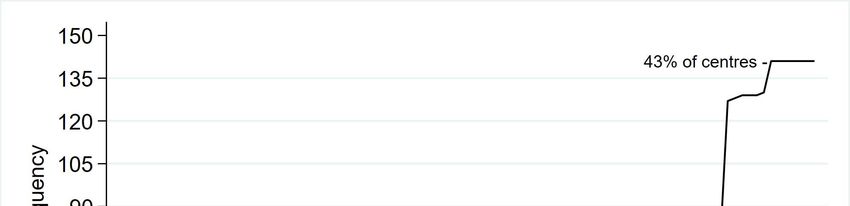
Exhibit 1 - Living Wage Treatments Over Time

Note: The figure reports the number of treated establishments over time. The figure only includes which
were treated while run by The Company. Some establishments were already subjected to the Living Wage
when taken over by The Company.

 21

Exhibit 2 - Wage and Hours Discontinuities

 (a) Wages (b) Hours

Note: The left and right figures respectively report log wages and log hours controlling for establishment and year-month fixed effects, by months relative to age 18 for 2 years before and after the cut-off,
for those treated and untreated with the Living Wage. The dashed line marks the age 18 cutoff. The sample is a panel of entry-level casual workers employed by The Company active between January 2011
and April 2019.

 22

Exhibit 3 – Wage and Hours Equations

 (1) (2) (3) (4)
 Log Wage Log Wage Log Casual Hours Log Casual Hours

 Eighteen X Treated 0.072 (0.015) 0.072 (0.015) -0.326 (0.102) -0.266 (0.093)
 Eighteen 0.121 (0.007) 0.128 (0.007) 0.097 (0.045) 0.166 (0.046)
 Treated 0.056 (0.015) 0.052 (0.014) 0.099 (0.126) 0.084 (0.125)
 Age/100 0.120 (0.037) -0.024 (0.048) -0.655 (0.314) -0.801 (0.504)
 Age/100 X Eighteen -0.143 (0.042) -0.007 (0.005) -.1.679 (0.427) -2.502 (0.631)
 Age/100 X Treated -0.057 (0.068) -0.090 (0.096) 1.472 (0.700) 0.381 (1.046)
 Age/100 X Eighteen X Treated 0.109 (0.082) 0.122 (0.120) -0.721 (0.940) 0.377 (1.325)

 Centre FE Yes Yes Yes Yes
 Year-Month FE Yes Yes Yes Yes

 Sample Size 94606 55176 94606 55176
 R2 0.740 0.754 0.179 0.180
 Window ±24 Months ±12 Months ±24 Months ±12 Months

Notes: The table reports parameter estimates from model (1) and (2) under different sample windows around the age 18 cut-off. Standard errors are clustered
at the establishment and are reported in parentheses.

 23

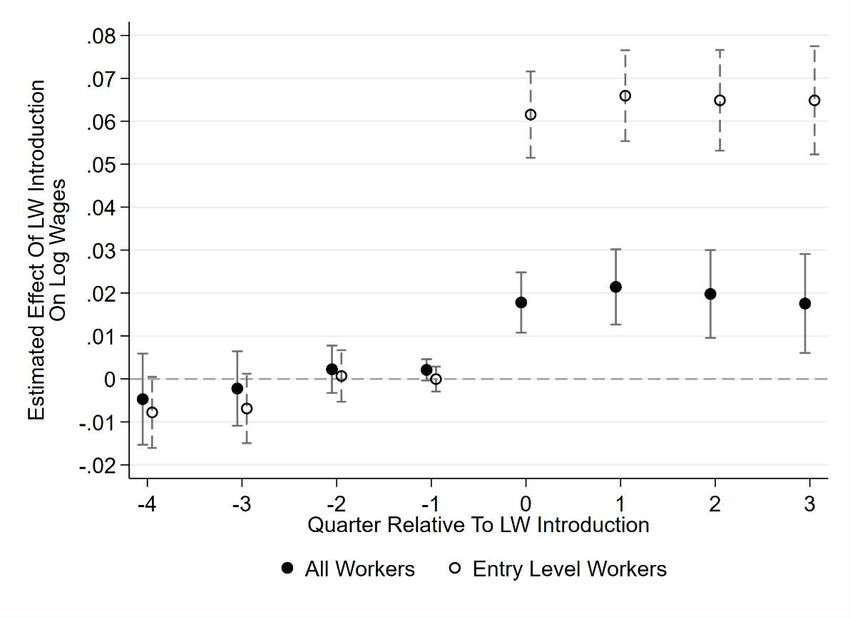
Exhibit 4 - Living Wage Effect on Total Casual Hours

Notes: The graph reports the estimates coefficient from model (6). The sample is a panel of
establishments run by The Company active between January 2011 and April 2019. The vertical bars
indicate 95% confidence intervals based on bootstrapped standard errors. Parameters are normalised to
month -1 and -12.

 24

Exhibit 5: Monopsony Market for 18 Year Olds

Notes: The figure presents a basic model of monopsony, with changes in the wage
due to changing age from just less than 18 (W

Online Appendix

 Additional Figures and Tables

 Figure A1: Living Wage Rates

Notes: The figure presents the hourly wage rate of the nationally mandated 21+ minimum wage (NMW
Adult rate), the 25+ minimum wage (NLW) and the Living Wage Foundation’s non-London UK rate
(UKLW) and the London rate (LLW).

 26

Figure A2: Living Wage Effect on Wages I

Notes: The graph reports the estimates coefficient from model (6). The sample is a panel of establishments
run by The Company active between January 2011 and April 2019. The vertical bars indicate 95%
confidence intervals based on bootstrapped standard errors. Parameters are normalised to month -1 and -
12.

 27

Figure A3: Living Wage Effect on Wages II

Notes: The graph reports the estimates coefficient from model (8). The sample is a panel of establishments
run by The Company active between January 2011 and April 2019. The vertical bars indicate 95%
confidence intervals based on bootstrapped standard errors. Parameters are normalised to month -1 and -
12.

 28

Table A1: Summary Statistics

 2019
 All Entry-level
 Mean S.D. Mean S.D.

Female 0.60 0.49 0.55 0.50
BAME 0.22 0.42 0.25 0.43
Age 35.94 14.31 31.43 13.86

Table A2: Event Study Estimates

 (1) (2) (3) (4) (5)
 log(casual hours) log(wage) log(wage) log(wage) log(wage)
Treated x Quarter
 -4 -0.070 (.049) 0.001 (.001) -0.002 (.002) -0.005 (.005) -0.008 (.004)
 -3 -0.086 (.065) 0.005 (.003) -0.002 (.003) -0.002 (.004) -0.007 (.004)
 -2 -0.108 (.080) 0.005 (.002) 0.003 (.002) 0.002 (.003) 0.001 (.003)
 -1 0.067 (.041) 0.002 (.001) 0.002 (.001) 0.002 (.001) 0.000 (.001)
 0 0.049 (.083) 0.016 (.003) 0.061 (.004) 0.018 (.004) 0.062 (.005)
 1 0.020 (.087) 0.019 (.003) 0.065 (.004) 0.021 (.004) 0.066 (.005)
 2 0.026 (.114) 0.016 (.004) 0.066 (.005) 0.020 (.005) 0.065 (.006)
 3 -0.076 (.115) 0.012 (.005) 0.065 (.006) 0.018 (.006) 0.065 (.006)

Centre FE Yes Yes Yes Yes Yes
Year-Month FE Yes Yes Yes Yes Yes

Sample Size 17,879 17,879 17,879 17,879 17,879
Estimating Equation (6) (6) (6) (8) (8)
Sample of Workers All All Entry-Level All Entry-Level

Notes: The table reports parameter estimates from model (6) for log(casual hours) and log(wages) and from model (8) for log(wages) for different samples of workers, and are
the counterpart estimates for Exhibit 4, Figure A2 and Figure A3. Columns (1), (2) and (3) report bootstrapped standard errors in parentheses and columns (4) and (5) report
standard errors clustered at the establishment in parentheses. Columns (2) and (4) include controls for the proportion of entry-level workers.

 30

CENTRE FOR ECONOMIC PERFORMANCE
 Recent Discussion Papers

1802 Holger Breinlich Trade, gravity and aggregation
 Dennis Novy
 J.M.C. Santos Silva

1801 Ari Bronsoler The impact of healthcare IT on clinical
 Joseph Doyle quality, productivity and workers
 John Van Reenen

1800 Italo Colantone The backlash of globalization
 Gianmarco Ottaviano
 Piero Stanig

1799 Jose Maria Barrero Internet access and its implications for
 Nicholas Bloom productivity, inequality and resilience
 Steven J. Davis

1798 Nicholas Bloom The diffusion of disruptive technologies
 Tarek Alexander Hassan
 Aakash Kalyani
 Josh Lerner
 Ahmed Tahoun

1797 Joe Fuller The demand for executive skills
 Stephen Hansen
 Tejas Ramdas
 Raffaella Sadun

1796 Stephen Michael Impink Communication within firms: evidence from
 Andrea Prat CEO turnovers
 Raffaella Sadun

1795 Katarzyna Bilicka Organizational capacity and profit shifting
 Daniela Scur

1794 Monica Langella Income and the desire to migrate
 Alan Manning

1793 Nicholas Bloom The donut effect of Covid-19 on cities
 Arjun Ramani

1792 Brian Bell This time is not so different: income dynamics
 Nicholas Bloom during the Covid-19 recession
 Jack Blundell

1791 Emanuel Ornelas Intra-bloc tariffs and preferential margins in
 Patricia Tovar trade agreements

1790 Jose Maria Barrero Why working from home will stick
 Nicholas Bloom
 Steven J. Davis

1789 Scott R. Baker What triggers stock market jumps?
 Nicholas Bloom
 Steven J. Davis
 Marco Sammon

1788 Nicolas Bloom The impact of Covid-19 on US firms
 Robert S. Fletcher
 Ethan Yeh

1787 Philippe Aghion Opposing firm-level responses to the China
 Antonin Bergeaud shock: horizontal competition versus vertical
 Matthieu Lequien relationships
 Marc J. Melitz
 Thomas Zuber

1786 Elsa Leromain Voting under threat: evidence from the 2020
 Gonzague Vannoorenberghe French local elections

1785 Benny Kleinman Dynamic spatial general equilibrium
 Ernest Liu
 Stephen J. Redding

1784 Antonin Bergeaud Technological change and domestic
 Clément Malgouyres outsourcing
 Clément Mazet-Sonilhac
 Sara Signorelli

1783 Facundo Albornoz Firm export responses to tariff hikes
 Irene Brambilla
 Emanuel Ornelas

 The Centre for Economic Performance Publications Unit
 Tel: +44 (0)20 7955 7673 Email info@cep.lse.ac.uk
 Website: http://cep.lse.ac.uk Twitter: @CEP_LSE