Machine Learning Project Paper: Group CERN
←
→
Page content transcription
If your browser does not render page correctly, please read the page content below
Machine Learning Project Paper: Group CERN
Cory Boatright, Erica Greene and Roman Shor

1     Introduction
We implemented a variety of techniques to improve classification of images and blogs by age and
gender for the Machine Learning 2009 competition. The starter files provided us a baseline imple-
mentations using simple versions of Naive Bayes for blogs and SVM for images. Blog classification
was improved by adding additional features to Naive Bayes and by stemming the dictionary of
unique words. Image classification was improved by moving to the HSV colorspace, introducing
Haar wavelets, and implementing PCA. Perceptron and generated typical faces where also investi-
gated before being discarded for low performance.

2     Blogs
2.1    Augmenting Naive Bayes
Our initial idea for improving the classification of the blogs was to add features to the Naive
Bayes classifier. The first feature we tried was average sentence length. The intuition was that
this feature would be helpful for age classification. We predicted adults would be less likely than
younger writers to use short fragmented sentences. There was also an article which found that
when average sentence length was paired with other features such as content words, it improved
classification for age and gender in blogs.[1] This result was encouraging because we already had
a set of features that took into account content words. What we found was that average sentence
length was not a strongly discriminative feature. Cross validation showed no improvement and the
feature took a long time to train and test. Part of the problem seemed to be ambiguity over what
defines the end of a sentence. Just using ‘.’, ‘!’, and ‘!’ missed many of the tokens we wanted to
consider as indicating the end of a sentence while allowing any word that includes the above three
symbols includes tokens that should not indicate the end of a sentence. Since we had a limited time
to work, we decided to abandon the idea.
    The next feature we added was average word length. While we were somewhat skeptical of
the potential of this feature, we found a number of articles that have found it useful in gender
classification for blogs. The implementation of this feature was significantly faster because we
made a key that mapped words in our dictionary to their length. This allowed us to do all the
preprocessing before training time and test time. We decided to turn average word length into a
binary feature and we chose the constant of 3.7. The feature was 0 if average word length was less
than 3.7 and it was one if average word length was greater than or equal to 3.7. We made a graph
that showed the difference of P (averagewordlength < constant|male) − P (averagewordlength <
constant|f emale) and a similar graph for age. Below is one of these graphs. It demonstrates why
we picked a constant of 3.7.

                                                1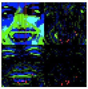
2 Blogs                                                                                         2

The average word feature was most useful for age as shown in the chart below.

                               P(Average Word Length | Age)
                                             13-17   23-27   33-47
                       Avg word length < 3.7 0.6305 0.3627 0.2917
                       Avg word length ≥ 3.7 0.3713 0.6384 0.7125
                             P(Average Word Length | Gender)
                                                 Male    Female
                          Avg word length < 3.7 0.3817 0.5095
                          Avg word length ≥ 3.7 0.6195 0.4917

    Although average word length seemed more promising, it also showed little improvement upon
testing. Perhaps adding it after pruning the number of features would have been more successful
because there would not be as much noise. If we were to do this project again, we would use PCA
or mutual information to significantly decrease the number of features before adding any new ones.
In the literature, many groups found that only a few hundred features gave comparable results to
using thousands of features.

2.2       Stemming
The original dictionary provided in the starter kit contained 80,000 words, each of which was
considered a feature in the overall classification. This dictionary was done in a nave manner, if
3 Images 3
a word existed in the training set it was included, so a lot of duplication existed. For example,
nouns and their plurals and all tenses of verbs were treated as separate features. Stemming tries to
mitigate this duplication by using an algorithm to reduce a word to its stem. The concept behind
this technique is that such parts of a word as the suffix and other minor variations can be peeled
off. This would remove the duplicate features. We used the Porter Stemmer Matlab code found
online. We discovered the code online as capable of crashing but only in rare degenerate cases, so
we caught those exceptions and handled them gracefully. The entire dictionary was converted into
a dictionary of stems, along with an index remapping that efficiently translated the blogs from their
original dictionary indices to the stemmed dictionarys indices. We did not clean the dictionary in
any way before generating the stems, and the resulting dictionary was 50,000 stems long. This
represents a 50% reduction in the dimensionality of the blogs themselves.
3 Images
3.1 Haar Wavelets and Colorspace
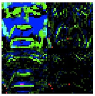
Fig. 1: Haar Wavelets of a typical male and female
This technique had amazing performance for gender. It was built in a piecemeal fashion to
simply beat the baselines. We knew we needed a better colorspace than RGB, so we experimented
with all the colorspaces available in the code from the starter kit. The best average improvement
over baseline was the HSV colorspace. We also knew that pixels were a poor choice of features due
to the high variability of the feature value from sample to sample. We wanted a way to consider
sets of pixels at a time, and the most readily available algorithm for this is wavelets. We had code
for many different wavelets available in the starter kit, and tried a handful of them, the best of
which was Haar wavelets. Research online (wikipedia) showed this to be the most basic wavelet.
The wavelets work through averaging and then finding the difference from averages and recursively
doing this to each level. We thought this averaging and distance from average would be most
important for age classification, since wrinkles or age spots would affect these averages. The major
benefit proved to be in gender instead. We ran 30-fold cross-validation with a range of slack settings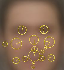
3 Images                                                                                           4

for the radial basis kernel, and the test set result was within 1% of the cross-validation result. We
have created images of what the images looked like after processing, granted these images are HSV
and recast directly into RGB (H = R, S = G, etc) so the colors resemble an Andy Warhol painting.
Typical wavelet features are shown in Figure 1.

3.2    PCA
We tried to reduce the dimensionality of the images with PCA, and only for the age classification.
While Matlab has a built-in PCA function, we did not have much success in learning how to actually
use it. Instead, we found a tutorial online about using another implementation of PCA with images
(http://www.cs.ait.ac.th/ mdailey/matlab/). This implementation was not only more intuitive to
use, but was also faster in execution and may have a smaller memory footprint. We looked at
the CDF for variability over increasing numbers of eigenvectors, but this graph grew too quickly
to be of much use. We instead used cross-validation to determine the most promising number of
dimensions to use. Using 30-fold cross-validation, we found 75 dimensions to be the most promising
result. We then experimented with both radial and polynomial kernels in LIBSVM and the total
combinations of parameters tested for polynomial kernels was approximately 3200. For degree 3,
coefficient 1, and slack amount 1, we were achieving a cross-validation score of 61.28% accuracy.
When submitted for running against the test set, we were reported to have an accuracy of less than
48.6%. A drop of this magnitude suggests some unknown bias in the testing or training set which
the dimensionality reduction was not able to take into account.

3.3    Perceptron
In the search for another approach to image classification, using a perceptron was initially investi-
gated. All images were subjected to the same dimensionality reduction that the baseline svm used,
and a similar random fold cross validation test procedure was used. The resulting accuracy was just
over 72% even with varied learning rates, so it was quickly abandoned in favor of Haar wavelets.
Due to the binary nature of perceptron, no serious attempts were undertaken to implement it for
age classification, even though a preliminary binary run had accuracies over 40%.

3.4    Average Faces
We found an interesting instance based method to implement that involved the modeling of an
average face from the training data (shown in Figure 2) and classification based on the average.
The average was generated with a simple average of all the pixels in the image which generated a
washed out, yet recognizable face. Curiously, the average male wears a suit and has a surprising
resemblance to George Bush. Features that can immediately be distinguished as unique to each
are the curvature of the mouth, the cheekbones, the eyes, and the hair. However, implementing a
classifier that could recognize these features proved difficult. The average images themselves are
blurry and washed out which contributes to their ambiguity.
    The scale invariant feature transform (SIFT) functionality of the VLFeat Matlab library was
used in an attempt to find features in the average faces and find a quantitative measure of how
close a test image was to the average. This measure was then used to classify images by gender
with a cross validation score of around 65%. The average faces when segregated by gender did not
produce any significant features when averaged naively. This method would have benefited greatly
3 Images 5
Fig. 2: Average male and female faces constructed from the entire training set (top). Features
extracted by the vlfeat toolkit (bottom)4 Conclusion 6
from a more robust method of generating average faces, and thus remains an interesting topic for
discussion.
4 Conclusion
After numerous test-time crashes and disappointing classifiers, we were finally able to beat the
baseline in all four categories. We tied for first place in the overall competition and we also had the
best accuracy for classifying images by age.
References
[1] Goswami, Sarkar, Rustagi 2009. Stylometric Analysis of Bloggers Age and Gender. Proceedings
of the Third International ICWSM Conference 2009.
[2] Schler, J., Koppel, M., Argamon, S., & Pennebaker, J. (2006, Spring). Effects of age and gender
on blogging.
[3] J.D. Burger and J.C. Henderson, 2006. An exploration of observable features related to blogger
age, In: Computational Approaches to Analyzing Weblogs: Papers from the 2006 AAAI Spring
Symposium. Menlo Park, Calif.: AAAI Press, pp. 1520.
[4] Burton, Mike and Jenkins, Rob. Averages : Recognising faces across realistic variation.
http://www.psy.gla.ac.uk/ mike/averages.html
[5] Takuya KAWANO, Kunihito KATO, Kazuhiko YAMAMOTO. A Comparison of the Gender
Differentiation Capability between Facial Parts. Proceedings of the 17th International Confer-
ence on Pattern Recognition. 2004.You can also read