Motion Sensor Monitoring and Ability Evaluation of Sprint Hurdle Swing Training under the Background of Wireless Communication Network

Hindawi
Mobile Information Systems
Volume 2021, Article ID 4679090, 13 pages
https://doi.org/10.1155/2021/4679090

Research Article
Motion Sensor Monitoring and Ability Evaluation of Sprint
Hurdle Swing Training under the Background of Wireless
Communication Network

 1
 Changliang Huang and Yuting Xu2
 1
 School of Competitive Sports and Physical Education, Shandong Sport University, Rizhao 276800, Shandong, China
 2
 School of Physical Education Department, Harbin Institute of Technology (Weihai), Weihai 264209, Shandong, China

 Correspondence should be addressed to Changliang Huang; huangchangliang@sdpei.edu.cn

 Received 11 August 2021; Revised 15 September 2021; Accepted 23 September 2021; Published 1 October 2021

 Academic Editor: Sang-Bing Tsai

 Copyright © 2021 Changliang Huang and Yuting Xu. This is an open access article distributed under the Creative Commons
 Attribution License, which permits unrestricted use, distribution, and reproduction in any medium, provided the original work is
 properly cited.
 The struggle with obstacles has very high technical requirements, and technical movements are particularly complex, requiring the
 coordination of the entire body of athletes. This article aims to study the training methods and training plans of sprinters, trying to
 gradually improve the waist strength, abdomen, and hip muscles of sprinters. Through basic strength training, we improve the
 ability of the body to coordinate strength and give full play to the core strength and sprint technique of the athletes. This paper
 proposes a motion sensor detection technology, which provides an effective tool for testing and analysis of sports training. The
 research object of this article is the hurdle running special physical speed, quality, and training methods. Based on a large amount
 of literature and theoretical analysis, an experimental group and a control group are set up, and an inductive analysis is carried out.
 The four aspects of peak power and half squat 1RM are discussed and analyzed in detail. The experimental results in this paper
 show that the extensor muscles of the experimental group increased by 56.5 J and 51.55 J, respectively, and the increase rates were
 24.72% and 19.66%, respectively. In the control group, the extensor muscles increased by 85 J and 52 J under the test conditions of
 60°/s and 300°/s, respectively, with an increase rate of 38.2% and 51.2%, respectively; the flexors increased by 32.6 J and 22 J,
 respectively, with an increase rate of 36.25% and 37.28%, respectively.

1. Introduction network [1]. Simply put, the wireless dynamic sensor net-
 work is to add dynamic nodes on the basis of the wireless
1.1. Background. The pace of technological development is sensor network. The dynamic node is based on the original
accelerating, and mankind has entered the information age. node of the wireless network sensor, adding a motion
As the most important and basic information acquisition control part, which will cause the initial static node to move
technology, sensor technology has also been developed by and add many new functions. The wireless dynamic sensor
leaps and bounds. Sensor information technology gradually network is the most advanced technology in the wireless
develops from simplification to integration. Since the end of sensor network.
the last century, fieldbus technology has been applied to
sensor networks. People use it to create smart sensor net-
works. A large number of multifunctional sensors are used 1.2. Significance. On the one hand, sensor network tech-
and connected through wireless technology, and wireless nology is a new type of network technology that incorporates
sensor networks are gradually taking shape. As the wireless radio communication technology. Sensor technology,
sensor network enters people’s lives, people put forward MEMS technology, and distributed information processing
higher requirements for the wireless sensor network, which technology are intercepting radio sensor networks. The
promotes the dynamic development of the wireless sensor information of the objects or environment in the monitoring

2 Mobile Information Systems

area are collected and processed through node cooperation; season training of Rugby Union players [4]. Gil and Lee
the processed information are transmitted to the end-users proposed to reduce the athlete’s personal recording time by
of the target network. Wireless sensor networks are widely applying the seven-step method. The authors conducted a
used, not only in the fields of environmental science and kinematic analysis of the seven-step method and the gen-
military but also in the field of daily medical care, smart erally accepted eight-step method of the current Korean
homes, and other commercial areas. On the other hand, hurdle record holder (13.43 s) and reached a conclusion
there is the meaning of sprint hurdles. From Liu Xiang’s gold about the seven-step method [5]. Misaki et al. proposed to
medal in the hurdle race at the Athens Olympics to the check the acceleration and deceleration curves of the ground
young player Xie Wenjun in the last 10 meters of the reaction force from the entire hurdle sprint to the fifth
Shanghai Athletics Federation Diamond League, he over- hurdle. By analyzing the performance of four male college
takes his opponent and stands on the podium. China is in the hurdlers, the force applied between the four steps in the
sprint event. Sports performance is constantly improving. It interval of the hurdle sprint was obtained. The curves are
can be found that the improvement of sports performance is different, indicating that the role of each step in an interval is
not only limited to good technical aspects but also has a leap different [6]. Camacho-Cardenosa et al. analyzed the impact
in special physical training. The reason Chinese hurdles have of the new low-dose repetitive sprint training on short- and
a place in international track and field must have their own long-term physical performance of team sports athletes in
unique training methods and methods. Even so, we should hypoxia (RSH). By testing before and after 4 weeks of su-
continue to improve and summarize the future development pervised specific training and 2 weeks after stopping train-
of the project and in-depth analysis of the shortcomings of ing, it is concluded that lower dose repetitive sprint training
unilateral training. Dyskinesia is a phenomenon in which under hypoxic conditions can increase the maximum power
voluntary movement is excited, inhibited, or cannot be and sprint of the hypoxic group of team sports athletes times
controlled by the will. It is common in mental disorders, [7]. Although the analysis is well done, some theories do not
neurological diseases, and trauma. have practical significance. There are some problems with
 the viewpoints and methods used by these scholars in the
 research process.
1.3. Related Work. The development of motion sensor de-
tection technology provides an effective tool for testing and
analysis of sports training. Pinto et al. proposes a new 1.4. Innovation. The innovations of this article are as fol-
technical solution for marker-based human motion capture, lows. (1) The first is the innovation of the topic selection
called WirelessSyncroVision (WSV). The proposed solution angle. This article is a new perspective from the perspective
is to synchronize the image acquisition in the remote of topic selection. At present, there are not many researches
multicamera with the opening time of the active marker and that integrate wireless communication, sprint hurdles,
adopt a robust method called adaptive and robust syn- motion sensors, physical fitness, and training methods. It is
chronization (ARS), and finally, it can be extended to other of exploratory significance. (2) The second is the innovation
than PbD equipment, such as motion capture, motion of research methods. This paper proposes a sensor optimal
analysis, and remote sensing systems [2]. Holmstrup et al. placement algorithm, wireless sensor network positioning
examined the effect of an 8 week KBS intervention on algorithm, and amorphous algorithm. These algorithms are
sprinting for leisurely active women, compared with an used to study the monitoring and performance of motion
8 week intervention using a stiff leg deadlift (SDL). After sensors. In addition, setting up an experimental group and a
pretests measuring 30-meter sprint and reverse vertical jump control group for experiments has high theoretical value and
performance, participants were divided into KBS (n � 8) and exploratory significance. (3) The third is the innovation of
SDL (n � 10) groups according to the sprint time. After project practice. The conclusions drawn can provide better
getting familiar with the exercises, KBS met twice a week, services for track and field training practice, to provide
using Tabata intervals (20 s of work, 10 s of rest, and 8 certain theoretical guidance and practical application value
rounds) for swings, emphasizing fast and explosive rhythms. for the athletic fitness of track and field sprinters.
It is concluded that future research should seek to determine
the appropriate number and strength of KBS components 2. Related Research Technology
for sprint programming [3]. Dobbin et al. determined the
utility of running-only and rugby-specific intraseasonal 2.1. Sensor Optimal Placement Algorithm. With the rapid
sprint interval interventions among professional rugby development of precision manufacturing technology,
league players. The research method is to assign 31 pro- computer technology, and information processing tech-
fessional college rugby players to rugby-specific (SITr/s, nology, increasingly sensors have been applied. When the
n � 16) or running-only (SITr, n � 15) sprint interval training information collected from each sensor is processed and
groups. The measurement of speed, strength, ability to isolated separately, not only the connection between the
change direction, prone yo-yo intermittent recovery test (yo- sensor information is interrupted but also the attributes of
yo IR1) performance, and heart rate recovery before and the relevant environment that may be contained in the
after the 2 week intervention, as well as the submaximal organic combination of information are also lost, which
response to prone yo-yo IR1, indicates that specific exercises leads to a waste of information resources and this leads to a
should be considered. The moves are incorporated into the high level of information processing. Information fusion

Mobile Information Systems 3

technology can effectively solve the above problems. It uses obtained and fused, and finally, the fusion information is
signal processing, artificial intelligence, mathematical sta- used as the evaluation criterion. The combination of
tistics, control principles and biology, and other related decision-making layers provides the best decision-mak-
theories to organically combine the local and incomplete ing and recognition performance but requires higher
sensory measurements of multiple sensors. These sensors are registration accuracy and sensor transmission bandwidth.
distributed in different positions and different states and use The fusion of the data layer retains as much original
complementary information to reduce data uncertainty and information as possible, but it also leads to greater in-
improve the accuracy and speed of multisensor systems [8]. formation processing and poor real-time performance.
 The workload of calculating the optimal position of the The merging of the feature layer is relatively simple,
measuring point is often relatively large, and most scholars compatible with the advantages and disadvantages of the
use the calculation software MATLAB programming [9] to decision layer [11] and the data layer [12] and provides
achieve. One of the most commonly used methods is the greater flexibility.
effective independence method, which calculates effective
independent vectors based on all possible measurement
points, sorts them according to the independence of the 2.2. Wireless Sensor Network Positioning Algorithm.
target modal matrix, and iteratively deletes the degrees of Mobile WSNs node positioning algorithms are mainly di-
freedom. vided into Monte-Carlo-based positioning algorithms, DV-
 Assuming that the number of all possible sensor posi- Hop positioning algorithms [13], and other positioning al-
tions is t and the number of sensors to be arranged is n, then gorithms. The Monte Carlo method, also known as the sta-
the response expression of the structure is tistical simulation method, refers to the use of random
 numbers (or more commonly pseudorandom numbers) to
 an � φn q + w, (1) solve many computational problems. The Monte Carlo
where a is the structural modal matrix. method is an essential type of numerical calculation method
 guided by the theory of probability and statistics, which was
 φn � φ1 , φ2 , . . . , φn � φij n ∗ t, (2) proposed in the mid-1940s due to the development of science
 and technology and the invention of electronic computers.
where φ1 � (φ1I , φ2I , . . . , φsI )T represents the I modal On this basis, people have proposed many improved posi-
vector; p � (p1 p2 . . . pt ) is the generalized coordinate; Q is tioning algorithms such as MCB, MSL, WMCL, and so on.
Gaussian white noise with a variance of η2 5. WSN data collection is shown in Figure 1.
 The least-squares estimation expression of modal co- The DV-Hop positioning algorithm [14] is mainly di-
ordinates is as follows: vided into three stages as follows. (1) The first stage obtains
 −1 the minimum number of hops. When the vector distance
 � φT n φn φT n us .
 p (3)
 exchange law is used to obtain the replacement condition of
 The covariance expression of the estimated error of p � the anchor node information, the corresponding hop
(p1 p2 . . . pt ) is as follows: number information is obtained. After that, the broadcast
 Internet and other media are used for information output,
 −1
 − p)T � z2 φT n φn .
 − p)(p
 U � L (p (4) such as the identification of the anchor node [15]. (2) The
 average hop distance between nodes is obtained in the
 Let P � φT n φn , P call the Fisher information matrix. It second stage. The following equation can be uses to calculate
can be seen from the Fisher information matrix that the the final result:
smaller the value of the covariance of the estimation error, �����������������
 2
the larger the value of the Fisher information matrix P, that i≠j hi − hj + ki − kj 
 (6)
is, when the matrix P norm takes the maximum value, the HopSizei � ,
 i≠j vij
estimate of p is the best estimate. The matrix P can be
expressed as follows: where vij refers to the minimum number of hops between
 n
 T
 s anchor nodes i(hi kj ) and j(hi kj ) 3. After calculating the
 P � φin φin � Pi . (5) average hop-per-hop distance of the anchor node, the data is
 i�1 i�1 corrected through broadcast information, and other values
 In the decision-level fusion process, the sensors need to are discarded after the unknown node has known the first
be transformed to obtain independent identity estimation, correction value.
and then the attributes of each sensor are classified and ai � HopSizei × kij . (7)
fused. In the process of data fusion [10], the original data
sent by sensors of the same size are directly merged, and then (3) Coordinate position calculation: The minimum
the merged data is analyzed and the feature extracted, and number and average jump distance measured before the
finally, the identity is determined according to the extracted calculation; the average distance and the unknown node to
features. In the feature-level fusion process, features are the anchor node are calculated; then obtain the number of
extracted by analyzing the output information of each sensor multiple nodes to obtain the least square node coordinates
so that the feature quantity of each observation target is [16].

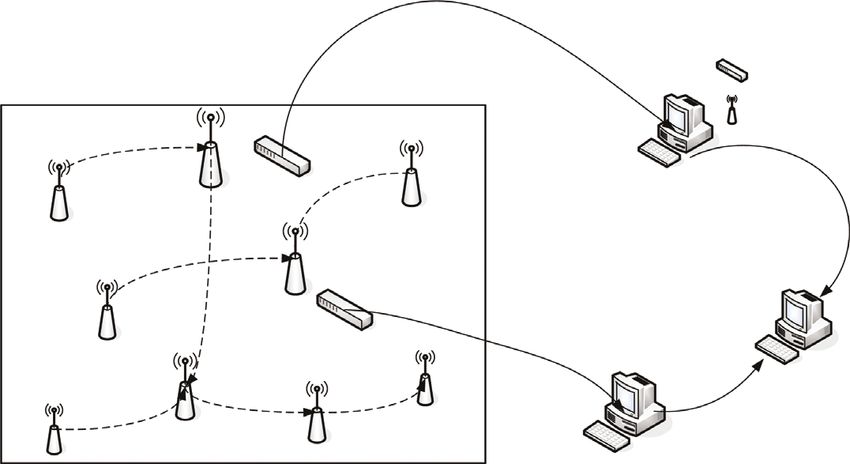
4 Mobile Information Systems

 the standard or the number of samplings is reached,
 this stage is stopped. The filter fusion block diagram
 Monitoring is shown in Figure 2:
 node
 Network (iii) Positioning stage (coordinate calculation): The
 node position coordinates of the unknown node at the
 Monitoring
 workstation moment are calculated by the following formula:
 m1
 W
 hit
 summary ht � ,
 workstation
 i�1
 W
 m0 (13)
 W
 ki
 Monitoring kt � t .
 workstation i�1
 W
 Figure 1: WSN data collection.

 The schematic diagram of the Monte Carlo algorithm is
 D1 + D3 shown in Figure 3:
 HopSizex � , (8)
 3+7
 D1 + D2 2.3. Amorphous Algorithm
 HopSizey � , (9)
 3+9
 2.3.1. Solve the Minimum Number of Hops. All anchor nodes
 D2 + D3 broadcast their location information to the entire network so
 HopSizez � . (10) that all nodes can receive this information, and the mini-
 7+8
 mum integer hops from each anchor node [19]; the mini-
 Using the principle of DV-HOP operation and posi- mum number of hops from node i to m can be calculated by
tioning, three average hop distances are obtained, and the the following formula:
three terms are the distances from the unknown node O to x,
y, and z, and then the least-squares method is used above to j∈nbrs(i) t(j, t)
 Q(i,m) � − 0.8. (14)
obtain the specific unknown node O coordinate. |nbrs(i)| + 1
 The MCL algorithm is a self-localization method for
 All anchor nodes broadcast their own location infor-
probability estimation based on Bayesian filtering. Its core
 mation to the whole network so that all nodes can receive
idea is to use a sample set Bt � (cit , fit )|i � 1, 2, . . . , W 
 this information and get the minimum integer jump [20]
containing W samples to estimate the posterior probability
 from each anchor node, m, i and the number of nodes from
[17]. Distribution Bt is the sample set at time t, cit is the first i
 m to i can be calculated by using formula (14).
samples, fit is the weight parameter, and the algorithm has
four steps in total. In prediction stage, at time t − 1, the node
position is clear, and then the position distribution of the
 2.3.2. Solve the Distance between Nodes. Equation (2) can be
node at time t has the following formula:
 used to calculate the average distance of each hop as follows:
 n √�����
 ⎨ 1/ πv2max , d ct−1 , ct < vmax
 ⎧ 2 ar cos t − t 1 − t2 
 k ct |ct−1 � ⎩ (11) HopSize � f⎛ ⎝1 + c − sπ
 − n ⎠.
 sa⎞
 0, d ct−1 , ct ≥ vmax −2

 (15)
 (i) Filtering stage: In the filtering stage of the algo-
 rithm [18], the main work is to filter out the Then the distance p between the unknown node and the
 sample points that do not meet the filtering anchor node is calculated using the minimum number of
 conditions. If W is a one-hop anchor node set, D hops calculated by the average distance of each hop that has
 represents a two-hop anchor node set, x is the been calculated above as follows:
 communication radius of the anchor node, z is the p � HopSizei × C(i,j) . (16)
 sample particle, and y is the anchor node.
 As long as the unknown node [21] finds the estimated
 filter(l) � (∀y ∈ Y, d(l, y) ≤ x) ∩ (∀y ∈ D, x < d(l, y) ≤ 2x).
 distance to the three anchor nodes, the following equations
 (12) can be listed to calculate the node coordinates:
 2 2
 (ii) Re-sampling: When the last stage is over, the ⎪
 ⎧
 ⎪
 ⎪ h − h + j1 − j � p21
 ⎨ 1
 number of remaining sample points may be less ⋮ , (17)
 ⎪
 ⎪
 than W, so the prediction process and filtering stage ⎪
 ⎩ 2 2 2
 must be re-executed. When the sample set reaches hn − h + jn − j � pn

Mobile Information Systems 5

 Reference sensor

 Main filter

 PM1
 Z1
 Sensor 1 Local filter 1

 Time update
 PM2

 Z2 Xg Xm
 Sensor 2 Local filter 2

 Optimal
 PMN
 integration

 ZN
 Sensor N Local filter N

 Figure 2: Block diagram of filter fusion.

 ⎪
 ⎧
 ⎪ h2 − h2n + j21 − j2n + p2n − p21
 ⎨ 1
 r s �⎪ ⋮ (20)
 ⎪
 ⎩ 2
 Y1 hn−1 − h2n + j2n−1 − j2n + p2n − p2n−1
 P1
 2r Finally, we use equations (17)–(20) to find the coordi-
 c1 P2 Y2
 nates of the unknown node.
 vmax

 3. Experimental Design of Sprint Hurdle Swing
 Y3 Training Based on Wireless Sensors
 3.1. Subjects. Eighteen men were selected as subjects of track
 and field sprint events. The average training level of all
 subjects reached the national athlete level 2. They are in good
 physical condition, have no injuries such as broken bones or
 muscle tears, and have no experience in vibration strength
 training. The 18 subjects were randomly divided into a test
 Figure 3: Schematic diagram of Monte Carlo algorithm. group (9) and a control group (9). The test group received
 vibration training, and the control group received con-
 where (h1 , j1 ), (h2 , j2 ), (h3 , j3 ), . . . , (hn , jn ) is the coor- ventional strength training.
dinates of anchor nodes, (h, j) is the coordinates of the To test whether there is a difference between the test
unknown node, and the distance between the unknown indicators of the test group and the control group before the
node and the anchor node is p1 , p2 , p3 , . . . , pn , respectively. test, the physical condition of the subjects and the four
 Then the above equations are solved according to the quality indicators are calculated as the quality indicators of
principle of the least-squares method, and then the specific 50 m sprint performance, knee flexion height, anaerobic
coordinates of the unknown nodes can be obtained as peak performance, and half squat 1RM. The test and analysis
follows: results are shown in Tables 1 and 2:
 Table 1 shows the statistical results of the physical
 −1
 Q � DT D DT n, (18) function indicators of the test group and the control group.
 The P-value of 0.365 of the age statistics of the test group and
 4 h1 − hn 4 j1 − jn the control group indicates that the age of the test group and
 ⎜
 ⎛ the control group is different. There was no significant
 W �⎜
 ⎜
 ⎜
 ⎝ ⋮ , (19)
 difference between the test group and the control group. The
 4 hn−1 − hn 4 jn−1 − jn experimental results show that P is 0.896, indicating that

6 Mobile Information Systems

there is no significant difference between the two. The Table 1: Pre-experiment information statistics of subjects in the
P-value of the weight statistics result is 0.875, which indi- experimental group and control group.
cates that there is no significant difference in weight between Group (n � 9) Age Height (cm) Weight (kg)
the experimental group and the control group. Test group 22.74 ± 1.46 182.42 ± 2.97 76.26 ± 7.52
 From Table 2, we can see the statistical results of the four Control group 23.68 ± 1.77 172.25 ± 6.78 78.23 ± 5.23
physical fitness indicators of the experimental and the control P-value 0.365 0.896 0.875
groups: the P-value of the 30-meter sprint performance of the
experimental and the control groups is 0.523. It shows that the
test and the control groups have no significant difference in Table 2: Statistics of the first four physical fitness indicators of the
30 m sprayable [22] energy; the statistical result of the knee experimental group and the control group.
joint level of the test and the control groups is 0.309 (P > 0.05),
 Index Test group Control group P-value
indicating that the knee joint level of the test and the control
groups has no jump height significant difference; the P-value of 30 m sprint (s) 3.106 ± 0.256 3.256 ± 0.026 0.523
 Squat jump height
the anaerobic peak performance statistics of the experimental 62.35 ± 6.23 62.35 ± 3.86 0.309
 (cm)
group and the control group is 0.268, indicating that there is no Anaerobic peak power
significant difference in the anaerobic peak performance of the 923.56 ± 116.25 902.36 ± 96.42 0.268
 (w)
experimental and the control groups. It includes that there is no Half squat 1RM (kg) 105.36 ± 6.38 156.48 ± 7.59 0.879
significant difference between the experimental and the control
groups. Tables 1 and 2 can be concluded that there is no
significant difference in physical fitness between the test and content was the same for 12 weeks, and each training session
the control groups, indicating that the test and the control lasted 120 min. The methods used in the control group are
groups meet the test conditions. relatively simplified and involve few steps, while the methods
 used in the experimental group are more diversified and
 detailed.
3.2. Training Program
3.2.1. Training Program of the Experimental Group. 3.3. Experimental Content
According to the principle of step-by-step training, when
athletes learn new skills and movements, they must follow 3.3.1. Training Content of the Experimental Group. The basic
the scientific logic system and the law of development of stage of core strength training is mainly to do some static
athletes’ understanding, from shallow to deep, from easy to movements on the sponge pad to improve the strength
difficult, and from simple to complex. The core strength quality of the small waist and abdomen muscles, initially
training studied in this article is an unfamiliar training develop the ability of the neuro-muscular system, and lay the
method for experimental subjects. To help athletes master foundation for the later core strength training. The ques-
the training method within a limited time, according to the tionnaire survey by experts shows that the training methods
principle of gradual training, the core strength training of and scores suitable for this stage are shown in Table 3:
this research is divided into three training stages: core Training plan: each training session adopts the cyclic
strength training basics phase, core strength training con- practice method. Six training stations are set up in
solidation phase, and core strength training improvement sequence. Six stations are completed continuously as a
phase. The basic period is 2 to 3 weeks, and the training group; each station has an interval of 4 min; and each
intensity is relatively small. The purpose is to improve the group has an interval of 4 min. The three groups of
strength of the waist and abdomen small muscle groups and exercises A, B, and C are static exercises [24], and the
promote the ability of the nerve-muscle system. The con- average persistence time per test is 40.5 s, so each
solidation period is 4 to 5 weeks. The training intensity is training session takes 55 s for each group of exercises;
moderate; the purpose is to further improve the strength the two groups D and E are dynamic exercises; each
quality of the small waist and abdomen muscles [23], group exercises 15 times, e component left and right leg
strengthen the coordination ability of the nerve-muscle exercises, 5 times on each side, continuous completion.
system, and develop the body balance and stability ability. Experts’’ training situation for the consolidation phase
The improvement phase is 5 to 6 weeks, and the training of core strength training is shown in Table 4:
intensity is high. The purpose is to develop the ability of the
 The core strength training improvement phase is based
nervous system to control balance under unstable conditions
 on the consolidation phase and gradually increases the
and to improve the strength of the small muscle groups of
 difficulty of training, that is, reducing the support base,
the waist and abdomen.
 gradually increasing instability, gradually increasing
 the number of repetitions of dynamic movements, from
3.2.2. Training Program of the Control Group. While the one-dimensional movements to multi-dimensional
experimental group was performing core strength training, movements, and so on. The training plan still adopts
the control group used traditional strength training methods the cyclic practice method. Six training stations are set
for waist and abdominal muscle training. The main up in sequence [25]; six consecutive stations are formed
equipment was sponge pads and barbells. The training as a group; the load of each group is 5 times; each

Mobile Information Systems 7

Table 3: Experts’ scores on training methods at the basic stage of Table 4: Experts’ ratings of training methods in the consolidation
core strength training. phase of core strength training.
 Average Training content Average score
Training content
 score Pull-in 4.5
Recumbent legs with arms stretched out and hips Hip extension and knee flexion 3.25
 3.25
straight Single-leg hip lift 4.2
Supine arm support hip lift leg lift 2.5 Reverse back extension 4.5
Side-up arms, hips, and legs 5
Side-lying banana pose from both ends 3.8
Lie on your back with one knee and hip 6 increase rate of 36.25% and 37.28%, respectively. The growth
 of extensor and flexor muscles has a very significant dif-
 station has an interval of 5 min; and each group has an ference within the group (P < 0.01); comparing the groups,
 interval of 6 min. the growth of the extensor muscles has a significant dif-
 ference, while the flexor muscles have no significant dif-
 ference, as shown in Figure 6:
3.3.2. Training Content of the Control Group. The control After the experiment, the relative peak torque of the knee
group used the traditional waist and abdomen strength joint flexors and extensors of the control and the experi-
training method and the circuit training method [26]; each mental groups increased to varying degrees. The knee joints
exercise was done in six groups; the training time and the of the experimental group were at 50°/s, 150°/s, and 200°/s.
number of training for each group are 15 reps and 25 Under the test conditions, the extensors increased by
seconds, such as supine and prone movements; the coach 1.32 Nm/kg, 1.35 Nm/kg, and 1.26 Nm/kg, respectively, and
makes each group do 25 reps or 25 seconds according to the the increase rate was 11.25%, 12.36%, and 14.36%, respec-
athlete's state. The training situation is shown in Table 5: tively, while the knee flexors increased by 1.25 Nm/kg,
 1.17 Nm/kg, and 1.19 Nm/kg, respectively, and the increase
4. Experimental Analysis rate was 20.3%, 23.56%, and 22.6%, respectively. Comparing
 the same group before and after the experiment, there was
4.1. Analysis of Experimental Results. After 10 weeks of
 no significant difference in the growth of the extensor and
training, the performance of the experimental group was
 the flexor muscle groups between two groups. Under the test
greatly improved compared with the control group. The
 conditions of 100°/s, 150°/s, and 200°/s, the extensors in-
1RM modification rate of the experimental group was higher
 creased by 1.2 Nm/kg, 1.5 Nm/kg, and 1.3 Nm/kg, respec-
than that of the control group, but there was no significant
 tively, with an increase rate of 25.6%, 25.36%, and 27.3%,
difference. After 8 weeks of training, the vibration training
 respectively. Muscle increased by 1.3 Nm/kg, 1.56 Nm/kg,
group recorded a significant increase in the 1RM of the half-
 and 1.2 Nm/kg, respectively, and the increase was 15.36%,
knee joint and a significant improvement. The increase in
 20.7%, and 20.14%, respectively. Comparing the same group
knee flexion of the experimental group was greater than that
 before and after the experiment, there is a significant dif-
of the control group, but there was no significant difference.
 ference in the growth of the extensor muscle group at 50°/s
The increase in peak anaerobic strength of the experimental
 and 200°/s, while the growth of the flexor muscle group at
group was greater than that of the control group, but there
 150°/s and 200°/s has a significant difference. Comparing
was no significant difference. The comparison of 50-meter
 between groups, there is a significant difference in the
sprint, half-knee maximum strength, knee height, and peak
 growth of the extensor muscle group at 200°/s, while the
anaerobic strength are shown in Figures 4 and 5.
 growth of the flexor muscle group at 150°/s has a significant
 difference, as shown in Figure 7:
4.2. Comparative Analysis of Peak Moments of Hip and Knee
Joints. The maximum work represents the maximum one-
time work value when a muscle group is repeatedly con- 4.3. Analysis of Related Technologies. The programming of
tracted for a certain number of times. It represents the the number of sensors optimization scheme is mainly
functional strength of the muscle and reflects the maximum based on the local minimum principle to select the
muscle strength to a certain extent. After the experiment, scheme. Therefore, the selection of the optimization
under the test conditions of 50°/s and 200°/s, the extensor scheme needs to be determined in conjunction with the
muscles of the experimental group increased by 56.5 J and maximum nondiagonal element change map of the MAC
51.55 J, respectively, and the increase rates were 24.72% and matrix. For the EI and MAC hybrid algorithm and the EI-
19.66%, respectively; the flexors increased by 20.36 J and 15 J, based stepwise subtraction method, since the algorithm
respectively, and the increase rates were 19.36% and 30.2%, itself has a reduced number of measurement points, there
respectively; there were significant differences in the growth may be only one local minimum. Under the condition of
of extensor and flexor muscles among the groups. In the selecting three sensors, the hybrid algorithm may have
control group, the extensor muscles increased by 85 J and only one or two minimum points. To facilitate compar-
52 J under the test conditions of 60°/s and 300°/s, respec- ison, the EI method uses the number of sensors deter-
tively, with an increase rate of 38.2% and 51.2%, respectively; mined by the stepwise accumulation method based on EI
the flexors increased by 32.6 J and 22 J, respectively, with an as a reference, and the hybrid algorithm of EI and MAC

8 Mobile Information Systems

 Table 5: Training content of lumbar and abdominal muscle strength training in the control group.
Training content Number of training groups Training times (times) Training time (s)
Sit-ups 6 25 20
Hanging leg lift 6 25 25
Lie on your back 6 25 25
Prone from both ends 6 25 25
Weight-bearing body flexion and extension 6 20 20
Prone “back leg” 6 25 20

 5000 150

 4500
 145

 4000
 140
 3500

 Maximum strength in a half squat
 135
 3000
 50 m sprint time

 2500 130

 2000
 125

 1500
 120
 1000

 115
 500

 0 110
 Control group test group Control group test group
 group group

 Before the experiment Before the experiment
 After the experiment After the experiment
 Figure 4: 50 m Sprint and half squat maximum strength comparison.

uses the number of sensors determined by the stepwise The measurement points selected by the effective in-
subtraction method as a reference. To facilitate the ob- dependent method achieve maximum linear independence,
servation of the six sensor optimization solutions corre- including orthogonality, and the selection range is greater
sponding to the maximum the changing law of than orthogonality. In the case of fewer sensor measurement
nondiagonal elements, the data are converted into a points, the measurement points selected by the effective
graph, as shown in Figure 8. independent method may not be able to take care of the
 It can be seen from Figure 8 that under the condition of installation of the sensor. When the added measurement
six sensors, the EI-based stepwise subtraction method points are better than orthogonal 45 in terms of linearity, the
proposed in this paper can achieve the best measurement phenomenon shown in Figure 9 will appear. The 16, 17, 145,
point layout effect. With the increase in the number of and 146 measuring points selected by the effective inde-
sensors, the measuring point arrangement scheme calcu- pendent method in this example have good linear inde-
lated by the gradual subtraction method presents a greater pendence, which can ensure that the vertical 1st and 2nd, 1st
advantage. The measuring point scheme provided by the EI and 4th, 3rd, and 4th orders have good positive values.
method also reflects the competitiveness in the case of However, the intersectionality cannot satisfy the orthogo-
multiple sensors. The gradual accumulation based on EI nality of the 2nd and 43rd, 3rd, and 6th orders, and the eight
proposed in this paper law is also competitive. At the same measuring points are adjacent to each other, resulting in a
time, it also shows that the number of sensors is not better, decrease in the degree of visualization of the measured mode
and a reasonable number of sensors need to be determined shape. Therefore, in the case of fewer sensor installation
comprehensively according to the actual needs. points, it is necessary to comprehensively consider the

Mobile Information Systems 9

 70 980

 960
 65
 940

 60 920
 Squat junp height (cm)

 50 m sprint time
 900
 55
 880

 50 860

 840
 45
 820

 40 800
 Control group test group Control group test group
 group group

 Before the experiment Before the experiment
 After the experiment After the experiment
 Figure 5: Comparison of squat jump height and anaerobic peak power.

 300 200

 250
 150
 200
 extensor muscles

 flexor muscles

 150 100

 100
 50
 50

 0 0
 200 50 200 50 200 50 200 50
 group (degrees/sec) group (degrees/sec)

 Before the experiment Before the experiment
 10 weeks later 10 weeks later
 Figure 6: Diagram of changes in the maximum work of the hip joint.

optimal placement of sensors through a variety of optimi- relatively large amount of calculation, and the number of
zation algorithms. The iteration times and maximum iterations is the same as the number of measuring points.
nondiagonal element changes of the two optimization al- Except for the effective independent method, several other
gorithms are shown in Figures 9 and 10. optimization algorithms converge quickly during the initial
 It can be seen from the figure that the effective inde- iteration process and can the local minimum be reached at
pendent method and the MAC hybrid algorithm have a five sensors.

10 Mobile Information Systems

 250 250

 100 100

 50 50
 group

 group
 250 250

 50 50

 100 100

 0 50 100 150 200 0 50 100 150 200 250
 peak extensor muscles peak extensor muscles

 percentage 10weeks later percentage 10weeks later
 Value-added Before the experiment Value-added Before the experiment
 Figure 7: Changes in peak torque of the knee joint group.

 1.2

 1
 largest non-diagonal element

 0.8

 0.6

 0.4

 0.2

 0
 0 1 2 3 4 5 6 7 8 9 10 11 12 13 14 15 16 17 18 19 20
 number of sensors

 EI algorithm MAC hybrid algorithm
 Stepwise accumulation method Stepwise subtraction
 Figure 8: The sensor optimization scheme corresponds to the change of the largest nondiagonal element.

Mobile Information Systems 11

 80

 70

 60

 50
 diagonal

 40

 30

 20

 10

 0
 0 1 2 3 4 5 6 7 8 9 10 11 12 13 14 15 16 17 18 19 20 21 22 23 24 25 26 27 28
 number of iterations

 EI method diagonal element change diagram
 Figure 9: Diagonal element change diagram of EI method.

 100

 90

 80

 70

 60
 diagonal

 50

 40

 30

 20

 10

 0
 0 1 2 3 4 5 6 7 8 9 10 11 12 13 14 15 16 17 18 19 20 21 22 23 24 25 26 27 28
 number of iterations

 MAC hybrid algorithm
 Figure 10: The maximum nondiagonal element change diagram of the EI and MAC hybrid algorithm.

5. Conclusions complete the software design; the motion state data are read
 with the upper machine; and the actual motion state in-
In this paper, the advantages and disadvantages of existing formation are compared. The sports performance of the
motion sensors are analyzed, and it has been finally decided world’s outstanding men’s 110-meter hurdles must be
to select six-axis three-degree-of-freedom sensing MPU6050 continuously improved. China’s hurdles have made
to detect the object motion state and select “amplitude- breakthrough progress in recent years, but there is still a
limited filtering algorithm + complementary filtering algo- certain gap compared with foreign outstanding athletes. The
rithm” to optimize and integrate the motion data, to im- average sports performance of Chinese athletes is much
prove the accuracy of motion state analysis. The main lower than that of high-level athletes in the world. This
research work in this paper is as follows: the “+ comple- directly reflects the lack of physical training of Chinese
mentary filter” algorithm is used to optimize the data and athletes. In particular, Chinese athletes are much worse than

12 Mobile Information Systems

foreign athletes in terms of speed quality. This is also a https://doi.org/10.1016/j.phycom.2020.101097 In press, Arti-
warning. We must continue to study and discover the cle ID 101097, 2020.
characteristics of athletes, conduct scientific and systematic [9] H. J. Lim, Y. J. Kang, and J. Y. Song, “Development of a mobile
analysis, and further improve the athlete’s speed quality. The game and wearable device for upper limb rehabilitation after
experimental results showed that the extensor muscles in the brain injury,” Journal of Rehabilitation Welfare Engineering &
 Assistive Technology, vol. 11, no. 3, pp. 253–259, 2017.
experimental group increased by 56.5j and 51.55j, respec-
 [10] D. Wu, D. Chatzigeorgiou, K. Youcef-Toumi, and R. Ben-
tively, with an increase rate of 24.72% and 19.66%, re- Mansour, “Node localization in robotic sensor networks for
spectively. The extensor muscle of the control group pipeline inspection,” IEEE transactions on industrial infor-
increased by 85j and 52j under the test conditions of 60°/s matics, vol. 12, no. 2, pp. 809–819, 2016.
and 300°/s, respectively, with the increase rates of 38.2% and [11] A. Philipose and A. Rajesh, “Investigation on energy efficient
51.2%, respectively; Flexor muscles increased by 32.6j and sensor node placement in railway systems,” Engineering
22j, respectively, with an increase rate of 36.25% and 37.28%, Science and Technology, an International Journal, vol. 19,
respectively. no. 2, pp. 754–768, 2016.
 [12] D. Wu, D. Chatzigeorgiou, K. Youcef-Toumi, and R. Ben-
 Mansour, “Node localization in robotic sensor networks for
Data Availability pipeline inspection,” IEEE Transactions on Industrial Infor-
 matics, vol. 12, no. 2, p. 1, 2016.
Data sharing is not applicable to this article as no data sets
 [13] S. Mukherjee, S. Nandy, and A. Dey, “Development of wildlife
were generated or analyzed during the current study. conservation system using energy-efficient real-time sensor
 networking,” International Journal of Engineering and Ad-
Conflicts of Interest vanced Technology, vol. 9, no. 4, pp. 866–874, 2020.
 [14] H.-W. Lee, J.-C. Chun, and W.-G. Jeong, “Removing the
The authors declare that there are no conflicts of interest motion artifacts in the pulse signal detected from the PFS
regarding the publication of this article. using the Quasi-periodicity,” Journal of Korea Institute of
 Information, Electronics, and Communication Technology,
 vol. 9, no. 6, pp. 591–598, 2016.
References [15] S. H. Hwang, K. R. Ko, and S. B. Pan, “Golf swing analysis
 [1] R. Parada, J. Melià-Seguı́, and R. Pous, “Anomaly detection system using camera and inertial sensor,” The Journal of
 using rfid-based information management in an IOTcontext,” Korean Institute of Information Technology, vol. 15, no. 4,
 Journal of Organizational and End User Computing, vol. 30, pp. 139–147, 2017.
 no. 3, pp. 1–23, 2018. [16] H. M. Do, H.-S. Kim, D. I. Park et al., “Intuitive teaching
 [2] A. M. Pinto, A. P. Moreira, and P. G. Costa, “Wire- device mountable on a robotic arm for efficient collaboration
 lessSyncroVision: wireless synchronization for industrial between humans and robots,” Journal of The Korean Society of
 stereoscopic systems,” International Journal of Advanced Manufacturing Technology Engineers, vol. 26, no. 6, pp. 577–
 Manufacturing Technology, vol. 82, no. 5–8, pp. 909–919, 2016. 583, 2017.
 [3] M. E. Holmstrup, B. T. Jensen, W. S. Evans, and [17] N. Kim, “A study on the implementation of transmission type
 E. C. Marshall, “Eight weeks of kettlebell swing training does PPG measurement device in a wrist watch,” Journal of Korea
 not improve sprint performance in recreationally active fe- Institute of Information, Electronics, and Communication
 males,” International Journal of Exercise Science, vol. 9, no. 3, Technology, vol. 10, no. 2, pp. 161–167, 2017.
 pp. 437–444, 2016. [18] C.-S. Kim and S.-H. Jung, “A MEMS-based finger wearable
 [4] N. Dobbin, J. Highton, S. L. Moss, and C. Twist, “The effects of computer input devices,” Journal of the Korea Institute of
 in-season, low-volume sprint interval training with and Information and Communication Engineering, vol. 20, no. 6,
 without sport-specific actions on the physical characteristics pp. 1103–1108, 2016.
 of elite academy rugby league players,” International Journal [19] Z. Y. Shi, “Application of motion capture technology based on
 of Sports Physiology and Performance, vol. 15, no. 5, MEMS sensor in sports training,” Revista de la Facultad de
 pp. 705–713, 2019. Ingenieria, vol. 32, no. 14, pp. 303–308, 2017.
 [5] H.-J. Gil and J.-H. Lee, “A study on the characteristics of [20] L. Lamprecht, R. Ehrenpfordt, T. Zoller, and
 110 m hurdle 7-step strategy: a pilot study,” Korean Journal of A. Zimmermann, “Application of human motion energy
 Sports Science, vol. 26, no. 3, pp. 1311–1320, 2017. harvesters on industrial linear technology,” IET Wireless
 [6] W. Misaki, S. Yasuo, R. Nagahara, A. Matsuo, and A. Nagano, Sensor Systems, vol. 9, no. 2, pp. 53–60, 2019.
 “Step-to-step analysis of anteroposterior ground reaction [21] J. Hanca, G. Braeckman, A. Munteanu, and W. Philips,
 force during 110 M hurdle,” ISBS Proceedings Archive, vol. 36, “Lightweight real-time error-resilient encoding of visual
 no. 1, p. 90, 2018. sensor data,” Journal of Real-Time Image Processing, vol. 12,
 [7] A. Camacho-Cardenosa, M. Camacho-Cardenosa, no. 4, pp. 1–15, 2014.
 I. Martı́nez-Guardado, J. Brazo-Sayavera, R. Timon, and [22] M. Haghi, K. Thurow, and R. Stoll, “A ubiquitous and con-
 G. Olcina, “Effects of repeated-sprint training in hypoxia on figurable wrist-worn sensor node in hazardous gases detec-
 physical performance of team sports players,” Revista Bra- tion,” Advances in Science, Technology and Engineering
 sileira de Medicina do Esporte, vol. 26, no. 2, pp. 153–157, Systems Journal, vol. 3, no. 5, pp. 248–257, 2018.
 2020. [23] I. Khoufi, P. Minet, A. Laouiti, and S. Mahfoudh, “Survey of
 [8] S. N. Mohanty, E. L. Lydia, M. Elhoseny, M. Majid, G. Al deployment algorithms in wireless sensor networks: coverage
 Otaibi, and K. Shankar, “Deep learning with LSTM based and connectivity issues and challenges,” International Journal
 distributed data mining model for energy efficient wireless of Autonomous and Adaptive Communications Systems,
 sensor networks,” Physical Communication, vol. 40, no. 3, vol. 10, no. 4, pp. 341–390, 2017.

Mobile Information Systems 13

[24] M. A. A. Mamun, M. A. Hannan, A. Hussain, and H. Basri,
 “Theoretical model and implementation of a real time in-
 telligent bin status monitoring system using rule based de-
 cision algorithms,” Expert Systems with Applications, vol. 48,
 pp. 76–88, 2016.
[25] X. Liu, M. Zhang, and V. Jan, “A low-power multifunctional
 CMOS sensor node for an electronic façade,” IEEE Trans-
 actions on Circuits & Systems I Regular Papers, vol. 61, no. 9,
 pp. 2550–2559, 2017.
[26] Y. Li and Y. Yang, “The research and implementation of
 dynamic loader for sensor network nodes,” Chinese Journal of
 Sensors and Actuators, vol. 31, no. 7, pp. 1113–1117, 2018.