Natural Language Processing with Deep Learning CS224N/Ling284 - Christopher Manning Lecture 3: Neural net learning: Gradients by hand matrix ...
←
→
Page content transcription
If your browser does not render page correctly, please read the page content below
Natural Language Processing
 with Deep Learning
 CS224N/Ling284

 Christopher Manning
Lecture 3: Neural net learning: Gradients by hand (matrix calculus)
 and algorithmically (the backpropagation algorithm)
1. Introduction
Assignment 2 is all about making sure you really understand the math of neural networks
… then we’ll let the software do it!

We’ll go through it all quickly today, but this is the week of quarter to most work through
the readings!

This will be a tough week for some! à
Make sure to get help if you need it
 Visit office hours
 Read tutorial materials given in the syllabus

Thursday will be mainly linguistics! Some people find that tough too
2
Named Entity Recognition (NER)
 • The task: find and classify names in text, for example:

 Last night , Paris Hilton wowed in a sequin gown .
 PER PER
 Samuel Quinn was arrested in the Hilton Hotel in Paris in April 1989 .
 PER PER LOC LOC LOC DATE DATE

 • Possible uses:
 • Tracking mentions of particular entities in documents
 • For question answering, answers are usually named entities
 • Often followed by Named Entity Linking/Canonicalization into Knowledge Base

3
Simple NER: Window classification using binary logistic classifier
• Idea: classify each word in its context window of neighboring words
• Train logistic classifier on hand-labeled data to classify center word {yes/no} for each
 class based on a concatenation of word vectors in a window
 • Really, we usually use multi-class softmax, but trying to keep it simple J
• Example: Classify “Paris” as +/– location in context of sentence with window length 2:

 the museums in Paris are amazing to see .

 Xwindow = [ xmuseums xin xParis xare xamazing ]T

• Resulting vector xwindow = x ∈ R5d , a column vector!
• To classify all words: run classifier for each class on the vector centered on each word
 in the sentence
4
NER: Binary classification for center word being location • We do supervised training and want high score if it’s a location 1 ! = = 1 + "# predicted model probability of class x = [ xmuseums xin xParis xare xamazing ] 5
Remember: Stochastic Gradient Descent
 Update equation:

 = step size or learning rate

 +, -
 i.e., for each parameter: $%&' = $()* −
 +-!"#$

 In deep learning, we update the data representation (e.g., word vectors) too!

 How can we compute ∇- ( )?
 1. By hand
 2. Algorithmically: the backpropagation algorithm
6
Lecture Plan
Lecture 4: Gradients by hand and algorithmically
1. Introduction (5 mins)
2. Matrix calculus (40 mins)
3. Backpropagation (35 mins)

7
Computing Gradients by Hand
• Matrix calculus: Fully vectorized gradients
 • “Multivariable calculus is just like single-variable calculus if you use matrices”
 • Much faster and more useful than non-vectorized gradients
 • But doing a non-vectorized gradient can be good for intuition; recall the first
 lecture for an example
 • Lecture notes and matrix calculus notes cover this material in more detail
 • You might also review Math 51, which has a new online textbook:
 http://web.stanford.edu/class/math51/textbook.html
 or maybe you’re luckier if you did Engr 108

8
Gradients
• Given a function with 1 output and 1 input
 = .
• It’s gradient (slope) is its derivative
 */
 *0
 = 3 1
 “How much will the output change if we change the input a bit?”
 At x = 1 it changes about 3 times as much: 1.013 = 1.03
 At x = 4 it changes about 48 times as much: 4.013 = 64.48

9
Gradients
 • Given a function with 1 output and n inputs

 • Its gradient is a vector of partial derivatives with
 respect to each input

10
Jacobian Matrix: Generalization of the Gradient
 • Given a function with m outputs and n inputs

 • It’s Jacobian is an m x n matrix of partial derivatives

11
Chain Rule
 • For composition of one-variable functions: multiply derivatives

 • For multiple variables at once: multiply Jacobians

12
Example Jacobian: Elementwise activation Function

13
Example Jacobian: Elementwise activation Function

 Function has n outputs and n inputs → n by n Jacobian

14
Example Jacobian: Elementwise activation Function

15
Example Jacobian: Elementwise activation Function

16
Example Jacobian: Elementwise activation Function

17
Other Jacobians

 • Compute these at home for practice!
 • Check your answers with the lecture notes
18
Other Jacobians

 • Compute these at home for practice!
 • Check your answers with the lecture notes
19
Other Jacobians

 Fine print: This is the correct Jacobian.
 Later we discuss the “shape convention”;
 using it the answer would be h.

 • Compute these at home for practice!
 • Check your answers with the lecture notes
20
Other Jacobians

 • Compute these at home for practice!
 • Check your answers with the lecture notes

21
Back to our Neural Net!

 x = [ xmuseums xin xParis xare xamazing ]
22
Back to our Neural Net!
 • Let’s find
 • Really, we care about the gradient of the loss Jt but we
 will compute the gradient of the score for simplicity

 x = [ xmuseums xin xParis xare xamazing ]
23
1. Break up equations into simple pieces

 Carefully define your variables and keep track of their dimensionality!
24
2. Apply the chain rule

25
2. Apply the chain rule

26
2. Apply the chain rule

27
2. Apply the chain rule

28
3. Write out the Jacobians

 Useful Jacobians from previous slide

29
3. Write out the Jacobians

 !

 Useful Jacobians from previous slide

30
3. Write out the Jacobians

 !

 Useful Jacobians from previous slide

31
3. Write out the Jacobians

 !

 Useful Jacobians from previous slide

32
3. Write out the Jacobians

 !
 !
 Useful Jacobians from previous slide

33
Re-using Computation

 • Suppose we now want to compute
 • Using the chain rule again:

34
Re-using Computation

 • Suppose we now want to compute
 • Using the chain rule again:

 The same! Let’s avoid duplicated computation …

35
Re-using Computation

 • Suppose we now want to compute
 • Using the chain rule again:

 !

 is the local error signal
36
Derivative with respect to Matrix: Output shape

 • What does look like?
 • 1 output, nm inputs: 1 by nm Jacobian?
 • Inconvenient to then do

37
Derivative with respect to Matrix: Output shape

 • What does look like?
 • 1 output, nm inputs: 1 by nm Jacobian?
 • Inconvenient to then do

 • Instead, we leave pure math and use the shape convention:
 the shape of the gradient is the shape of the parameters!

 • So is n by m:

38
Derivative with respect to Matrix

 • What is
 • is going to be in our answer
 • The other term should be because

 • Answer is:

 is local error signal at
 is local input signal

39
Deriving local input gradient in backprop
 "
• For " in our equation:

 = = ( + )

• Let’s consider the derivative of a single weight Wij
• Wij only contributes to zi u2
 • For example: W23 is only
 s
 used to compute z2 not z1 f(z1)= h1 h2 =f(z2)

 W23
 2
 = 23 + 2 b2
 2$ 2$
 +
 = ∑*567 25 5 = $ x1 x2 x3 +1
 +4%!
40
Why the Transposes?

• Hacky answer: this makes the dimensions work out!
 • Useful trick for checking your work!
• Full explanation in the lecture notes
 • Each input goes to each output – you want to get outer product
41
What shape should derivatives be?

 • Similarly, is a row vector
 • But shape convention says our gradient should be a column vector because b is
 a column vector …

 • Disagreement between Jacobian form (which makes the chain rule
 easy) and the shape convention (which makes implementing SGD easy)
 • We expect answers in the assignment to follow the shape convention
 • But Jacobian form is useful for computing the answers

42
What shape should derivatives be?
 Two options:
 1. Use Jacobian form as much as possible, reshape to
 follow the shape convention at the end:
 • What we just did. But at the end transpose to make the
 derivative a column vector, resulting in

 2. Always follow the shape convention
 • Look at dimensions to figure out when to transpose and/or
 reorder terms
 • The error message that arrives at a hidden layer has the
 same dimensionality as that hidden layer

43
3. Backpropagation

We’ve almost shown you backpropagation
 It’s taking derivatives and using the (generalized, multivariate, or matrix)
 chain rule
Other trick:
 We re-use derivatives computed for higher layers in computing
 derivatives for lower layers to minimize computation

44
Computation Graphs and Backpropagation • Software represents our neural net equations as a graph • Source nodes: inputs • Interior nodes: operations + 45
Computation Graphs and Backpropagation • Software represents our neural net equations as a graph • Source nodes: inputs • Interior nodes: operations • Edges pass along result of the operation + 46
Computation Graphs and Backpropagation • Software represents our neural net equations as a graph • Source nodes: inputs • “Forward Propagation” Interior nodes: operations • Edges pass along result of the operation + 47
Backpropagation • Then go backwards along edges • Pass along gradients + 48
Backpropagation: Single Node
 • Node receives an “upstream gradient”
 • Goal is to pass on the correct
 “downstream gradient”

 Downstream Upstream
49 gradient gradient
Backpropagation: Single Node

 • Each node has a local gradient
 • The gradient of its output with
 respect to its input

 Downstream Local Upstream
50 gradient gradient gradient
Backpropagation: Single Node

 • Each node has a local gradient
 • The gradient of its output with
 respect to its input

 Chain
 rule!
 Downstream Local Upstream
51 gradient gradient gradient
Backpropagation: Single Node

 • Each node has a local gradient
 • The gradient of its output with
 respect to its input

 • [downstream gradient] = [upstream gradient] x [local gradient]

 Downstream Local Upstream
52 gradient gradient gradient
Backpropagation: Single Node
 • What about nodes with multiple inputs?

 *

53
Backpropagation: Single Node
 • Multiple inputs → multiple local gradients

 *

 Downstream Local Upstream
 gradients gradients gradient
54
An Example

55
An Example

 Forward prop steps

 +

 *
 max

56
An Example

 Forward prop steps

 1

 2
 + 3

 6
 2 *
 2
 max
 0
57
An Example

 Forward prop steps Local gradients

 1

 2
 + 3

 6
 2 *
 2
 max
 0
58
An Example

 Forward prop steps Local gradients

 1

 2
 + 3

 6
 2 *
 2
 max
 0
59
An Example

 Forward prop steps Local gradients

 1

 2
 + 3

 6
 2 *
 2
 max
 0
60
An Example

 Forward prop steps Local gradients

 1

 2
 + 3

 6
 2 *
 2
 max
 0
61
An Example

 Forward prop steps Local gradients

 1

 2
 + 3
 1*2 = 2 6
 2 * 1
 2
 max 1*3 = 3
 0
 upstream * local = downstream
62
An Example

 Forward prop steps Local gradients

 1

 2
 + 3
 2
 6
 2 * 1
 2
 3*1 = 3
 max 3
 0
 3*0 = 0 upstream * local = downstream
63
An Example

 Forward prop steps Local gradients

 1
 2*1 = 2
 2
 + 3
 2
 2*1 = 2 6
 2 * 1
 2
 3
 max 3
 0
 0 upstream * local = downstream
64
An Example

 Forward prop steps Local gradients

 1
 2
 2
 + 3
 2
 2 6
 2 * 1
 2
 3
 max 3
 0
 0
65
Gradients sum at outward branches

 +

66
Gradients sum at outward branches

 +

67
Node Intuitions

 • + “distributes” the upstream gradient to each summand

 1
 2
 2
 + 3
 2
 2 6
 2 * 1
 2
 max
 0
68
Node Intuitions

 • + “distributes” the upstream gradient to each summand
 • max “routes” the upstream gradient

 1

 2
 + 3

 6
 2 * 1
 2
 3
 max 3
 0
 0
69
Node Intuitions

 • + “distributes” the upstream gradient
 • max “routes” the upstream gradient
 • * “switches” the upstream gradient

 1

 2
 + 3
 2
 6
 2 * 1
 2
 max 3
 0
70
Efficiency: compute all gradients at once • Incorrect way of doing backprop: • First compute * + 71
Efficiency: compute all gradients at once • Incorrect way of doing backprop: • First compute • Then independently compute • Duplicated computation! * + 72
Efficiency: compute all gradients at once • Correct way: • Compute all the gradients at once • Analogous to using when we computed gradients by hand * + 73
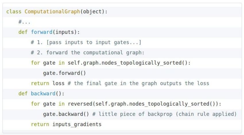
Back-Prop in General Computation Graph
 1. Fprop: visit nodes in topological sort order
 Single scalar output - Compute value of node given predecessors
 2. Bprop:
 - initialize output gradient = 1
 … - visit nodes in reverse order:
 Compute gradient wrt each node using
 gradient wrt successors
 … = successors of

 Done correctly, big O() complexity of fprop and
 bprop is the same
 … In general, our nets have regular layer-structure
 and so we can use matrices and Jacobians…
74
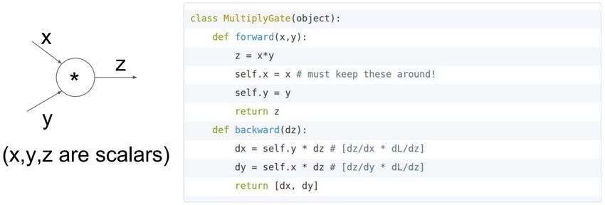
Automatic Differentiation

 • The gradient computation can be
 automatically inferred from the symbolic
 expression of the fprop
 • Each node type needs to know how to
 compute its output and how to compute
 the gradient wrt its inputs given the
 gradient wrt its output
 • Modern DL frameworks (Tensorflow,
 PyTorch, etc.) do backpropagation for
 you but mainly leave layer/node writer
 to hand-calculate the local derivative
75
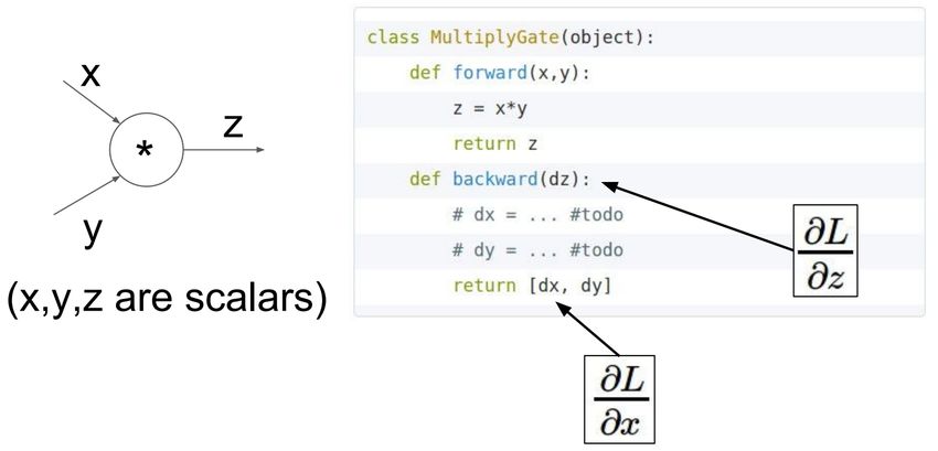
Backprop Implementations

76
Implementation: forward/backward API

77
Implementation: forward/backward API

78
Manual Gradient checking: Numeric Gradient

• For small h (≈ 1e-4),
• Easy to implement correctly
• But approximate and very slow:
 • You have to recompute f for every parameter of our model

• Useful for checking your implementation
 • In the old days, we hand-wrote everything, doing this everywhere was the key test
 • Now much less needed; you can use it to check layers are correctly implemented

79
Summary

We’ve mastered the core technology of neural nets!

• Backpropagation: recursively (and hence efficiently) apply the chain rule
 along computation graph
 • [downstream gradient] = [upstream gradient] x [local gradient]

• Forward pass: compute results of operations and save intermediate
 values
• Backward pass: apply chain rule to compute gradients
80
Why learn all these details about gradients?
• Modern deep learning frameworks compute gradients for you!
 • Come to the PyTorch introduction this Friday!

• But why take a class on compilers or systems when they are implemented for you?
 • Understanding what is going on under the hood is useful!

• Backpropagation doesn’t always work perfectly
 • Understanding why is crucial for debugging and improving models
 • See Karpathy article (in syllabus):
 • https://medium.com/@karpathy/yes-you-should-understand-backprop-e2f06eab496b
 • Example in future lecture: exploding and vanishing gradients

81
You can also read