Open-Set Face Recognition-based Visitor Interface System
←
→
Page content transcription
If your browser does not render page correctly, please read the page content below
Open-Set Face Recognition-based
                     Visitor Interface System

             Hazım K. Ekenel, Lorant Szasz-Toth, and Rainer Stiefelhagen

                  Computer Science Department, Universität Karlsruhe (TH)
                     Am Fasanengarten 5, Karlsruhe 76131, Germany
                            {ekenel,lszasz,stiefel}@ira.uka.de

       Abstract. This work presents a real-world, real-time video-based open-set face
       recognition system. The system has been developed as a visitor interface, where
       a visitor looks at the monitor to read the displayed message before knocking on
       the door. While the visitor is reading the welcome message, using the images
       captured by the webcam located on the screen, the developed face recognition
       system identifies the person without requiring explicit cooperation. According to
       the identity of the person, customized information about the host is conveyed. To
       evaluate the system’s performance in this application scenario, a face database
       has been collected in front of an office. The experimental results on the collected
       database show that the developed system can operate reliably under real-world
       conditions.

1 Introduction
Face recognition is one of the most addressed topics in computer vision and pattern
recognition research communities. Closed-set face identification problem, assigning
test images to a set of known subjects, and face verification, comparing test images
with the ones from claimed identity to check whether the claim is correct or not, have
been extensively studied. However, on open-set face recognition, determining whether
the encountered person is known or not and if the person is known finding out who he
is, there exists only a few studies [1, 2]. In [1] a transduction-based approach is intro-
duced. To reject a test sample, its k-nearest neighbors are used to derive a distribution
of credibility values for false classifications. Subsequently, the credibility of the test
sample is computed by iteratively assigning it to every class in the k-neighborhood. If
the highest achieved credibility does not exceed a certain level, defined by the previ-
ously computed distribution, the face is rejected as unknown. Otherwise, it is classified
accordingly. In [2] accumulated confidence scores are thresholded in order to perform
video-based open-set face recognition. It has been stated that in open-set face recog-
nition, determining whether the person is known or unknown is a more challenging
problem than determining who the person is.
     Open-set identification can be seen as the most generic form of face recognition
problem. Several approaches can be considered to solve it. One of them is to perform
verification and classification hierarchically, that is, to perform first verification to de-
termine whether the encountered person is known or unknown and then, if the person is
known, finding out who he is by doing classification (Fig. 1a). An alternative approach
can be training an unknown identity class and running just a classifier (Fig. 1b). A third
option is running just verifiers. A test image is compared against each known subject to
see whether it belongs to that subject or not (Fig. 1c). If all the verifiers reject, then the
image is classified as belonging to an unknown person. If one or more verifiers accept,
then the image is classified as belonging to a known person. Among these approaches,
we opt for the last one, which we name as the multi-verification approach. The main
reason for this choice is the better discrimination provided by the multi-verification ap-
proach. The first method requires a verifier to determine known/unknown persons. This
requires training the system with face images of known and unknown persons. Since
human faces are very similar, generating a single known/unknown verifier can not be
highly discriminative. In the second method, training a separate unknown class would
not be feasible, since the unknown class covers unlimited number of subjects that one
cannot model. On the other hand, with the multi-verification approach, only the avail-
able subjects are modeled. The discrimination is enhanced using the available data from
a set of unknown persons for support vector machine (SVM) based verifiers.
(a) Hierarchical (b) Classification-based
(c) Multiple verification
Fig. 1: Possible approaches for open-set face recognition
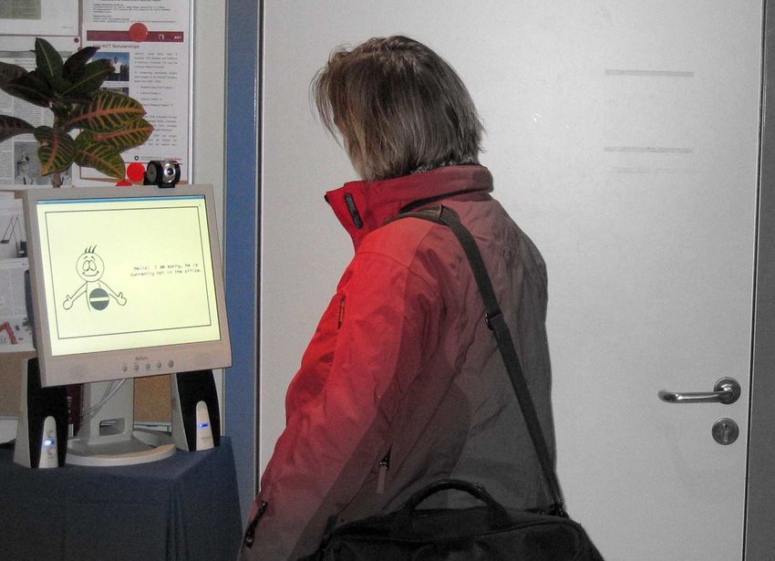
The system has been developed as a visitor interface, where a visitor looks at the
monitor before knocking on the door. A welcome message is displayed on the screen.
While the visitor is looking at the welcome message, the system identifies the visitor
unobtrusively without needing person’s cooperation. According to the identity of the
person, the system customizes the information that it conveys about the host. For exam-
ple, if the visitor is unknown, the system displays only availability information about
the host. On the other hand if the visitor is known, depending on the identity of the
person more detailed information about the host’s status is displayed. A snapshot of the
system in operation can be seen in Fig. 2.
Fig. 2: A snapshot of visitor interface in operation.

2 Open-set face recognition system

This section briefly explains the processing steps of the developed open-set face recog-
nition system.

2.1   Face Registration

In the system, faces are detected using Haar-like features based cascade of classifiers
[3]. Region-of-interest based face tracking is utilized to compensate misses in the face
detector. Eye detection is also based on cascade of classifiers [3]. Cascades were trained
for left and right eyes. They are then applied to detected face regions to find the eye
locations taking also anthropometric relationships into account. According to the eye
center positions the face is aligned and scaled to 64 × 64 pixels resolution.

Sample augmentation Imprecise registration reduces classification rate significantly.
In order to mitigate the effects of improper registration, for every available training
frame 25 additional samples are created by varying the detected eye positions for each
eye independently in the four-neighborhood of the original detection. When these posi-
tions are modified, the resulting aligned faces are slightly different in scale, rotation and
translation. Finally, the number of representatives are reduced to the original number of
samples by k-means clustering [2].

2.2   Face Representation

Face representation is done using local appearance-based face representation. There are
three main reasons to opt for this algorithm:

 – Local appearance modeling, in which a change in a local region affects only the
   features that are extracted from the corresponding block, while the features that are
   extracted from the other blocks remain unaffected.

– Data independent bases, which eliminate the need of subspace computation. In the
   case of real-world conditions, the variation in facial appearance is very high, which
   causes difficulty to construct suitable data-dependent subspaces.
 – Fast feature extraction using the discrete cosine transform (DCT), which enables
   real-time processing.
    This method can be summarized as follows: A detected and aligned face image is
divided into blocks of 8 × 8 pixels resolution. The DCT is applied on each block. Then,
the obtained DCT coefficients are ordered using zig-zag scan pattern. From the ordered
coefficients, M of them are selected and normalized according to a feature selection
and feature normalization strategy resulting in an M -dimensional local feature vector
[4]. In this study, we utilized M = 5 coefficients by leaving out the first coefficient
and using the following five coefficients. This local feature vector is then normalized
to unit norm. Finally, the feature vectors extracted from each block are concatenated to
construct the global feature vector. For details of the algorithm please see [4].

2.3   Verification
Support vector machines based verifiers are employed in the study [5]. Support vector
machines (SVMs) are maximum margin binary classifiers that solve a classification
task using a linear separating hyperplane in a high-dimensional projection-space. This
hyperplane is chosen to maximize the margin between positive and negative samples.
A polynomial kernel with degree 2 is used in this study. Confidence values are derived
directly from the sample’s distance-to-hyperplane, given a kernel K and the hyperplane
parameters w and b,
                                d(xi ) = K(w, xi ) + b.                             (1)

2.4   Multiple verification
As mentioned earlier, this work formulates the open-set face recognition problem as
a multiple verification task. An identity verifier is trained for each known subject in
the database. In testing, the test face image is presented to each verifier and N veri-
fications are performed, where N denotes the number of known subjects. If all of the
verifiers reject, the person is reported as unknown; if one accepts, the person is accepted
as known and the verified identity is assigned to him; if more than a single verifier ac-
cepts, the person is accepted as known and the identity of the verifier with the highest
confidence is assigned to him. Verifier confidences are inversely proportional to the
distance-to-hyperplane. Given a new sample x, a set of verifiers for every known sub-
ject {v1 , . . . , vN }, and a distance function d(vi , x) of sample x from subject i training
samples using classifier vi , the accepted identities are

                      identitiesx = {i|i ∈ [1 . . . n], d(vi , x) < t}.                   (2)

The best score is dx = min{d(vj , x)|j ∈ identitiesx } and the established identity is
id = argminj {d(vj , x)|j ∈ identitiesx }.
    For video-based identification, n-best match lists, where n ≤ N , are used. That is,
at each frame, every verifier outputs a confidence score and among these confidence
Table 1: Data organization for open-set face recognition experiments
                                    Training data
                      Known 5 subjects 4 sessions
                      Unknown 25 subjects 1 session
                                     Testing data
                      Known 5 subjects 3 – 7 sessions per person
                      Unknown 20 subjects 1 session per person

scores, only the first n of them having the highest confidence scores are accumulated.
Before the accumulation, the scores are first min-max-normalized so that the new score
value in the n-best list is
                                  si − smin
                     s′i = 1 −                      i = 1, 2, ..., n.                  (3)
                                 smax − smin
                                                              Pn      ′
Then, the scores are re-normalized to yield a sum of one,        i=1 si   = 1, in order to
ensure an equal contribution from each single video frame.

3 Evaluation

The data set consists of short video recordings of 54 subjects captured in front of an
office over four months. There is no control on the recording conditions. The sequences
consist of 150 consecutive frames where face and eyes are detected. Fig. 3 shows some
captured frames. As can be seen, the recording conditions can change significantly due
to lighting, motion blur, distance to camera and change of the view angle. For exam-
ple, as the subject comes closer to the system, his face will be tilted more to see the
interface. The subjects are assigned to two separate groups as known and unknown
subjects. The term known refers to the subjects that are added to the database during
training, whereas unknown refers to the subjects that are not added to the database.
Unless otherwise stated, in the experiments, five subjects, who are the members of a
research group, are classified as known people. 45 subjects who are mainly university
students and some external guests, are classified as unknown people. The recordings
of four additional subjects are reserved for the experiment, at which the effect of num-
ber of known subjects to the performance is analyzed. The set of recording sessions is
then further divided into training and testing data. Known subjects’ recordings are split
into non-overlapping training and testing sessions. From the 45 recordings of unknown
subjects, 25 are used for training and twenty of their recordings are used for testing.
The organization of the used data can be seen in Table 1. As can be noticed, for each
verifier training, there exists around 600 frames (4 sessions, 150 frames per session)
from the known subject. On the other hand, the number of available frames from the
unknown subjects is around 3750 frames (25 sessions, 150 frames per session). In order
to limit the influence of data imbalance during verifier training, unknown recordings are
undersampled to 30 images per used training session, making a total of 750 frames.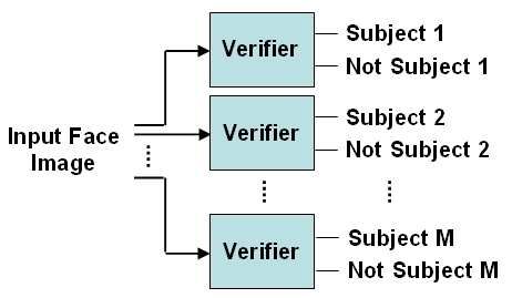
(a) Artificial     (b) Artificial   (c) Daylight,   (d) Daylight,
             light, far away    light, motion    brighter        darker
                                blur

                        Fig. 3: Sample images from the data set

    Open-set face recognition systems can make three different types of errors. False
classification rate (FCR) indicates the percentage of correctly accepted but misclassified
known subjects, whereas false rejection rate (FRR) shows the percentage of falsely
rejected known subjects and false acceptance rate (FAR) corresponds to the percentage
of falsely accepted unknown subjects. These three error terms have to be traded off
against each other in open-set face recognition by modifying a threshold and cannot be
minimized simultaneously. In the case of SVM-based verifier it is obtained by moving
the decision hyperplane. The equal error rate (EER) is defined as the point on the ROC
curve where F AR = F RR + F CR.

3.1   Frame-based verification

Frame-based verification implies doing verification using a single frame instead of an
image sequence. Each frame in the recordings is verified separately, that is, the decision
is taken only using a single frame at a time. The results of this experiment, at the closest
measurement point to the point of equal error, are reported in Table 2. In the table CCR
denotes the correct recognition rate and CRR denotes the correct rejection rate. The
threshold value used was ∆ = −0.12. The SVM classification is modified by shifting
hyperplane in parallel towards either class, so that the hyperplane equation becomes
wx + b = ∆.
     Obtained receiver operating characteristic (ROC) curve can be seen in Fig. 4. To an-
alyze the effect of FRR and FCR on the performance, they are plotted separately in the
figure. The dark gray colored region corresponds to the errors due to false known/unknown
separation and the light gray colored region corresponds to the errors due to misclassi-
fication. Similar to the finding in [2], it is observed that determining whether a person
is known or unknown is a more difficult problem than finding out who the person is.

                        Table 2: Frame-based verification results
                               CCR FRR FAR CRR FCR
                               90.9 % 8.6 % 8.5 % 91.5 % 0.5 %
1
0.9
0.8
Correct Classification Rate
0.7
0.6
0.5
0.4
0.3
0.2 FRR
FCR
0.1
EER
0
0.1 0.2 0.3 0.4 0.5 0.6 0.7 0.8 0.9 1
False Acceptance Rate
Fig. 4: ROC curve of frame-based verification
Table 3: Progressive score and video-based classification results
CCR FRR FAR CRR FCR
Frame 90.9 8.6 8.5 91.5 0.5
Progressive 99.5 0.5 0.1 99.9 0
Video 100 0 0 100 0
3.2 Video-based verification
As the data set consists of short video sequences, the additional information can be used
to further improve classification results. We evaluated two different cases. In the case of
progressive verification, the frames up to a certain instant, such as up to one second, two
seconds etc., are used and the decision is taken at that specific instant. The performance
is calculated by averaging the results obtained at each instant. In the case of video-based
verification, the decision is taken after using the frames of the entire video.
Table 3 shows the improved results with the help of accumulated scores. In both
cases the video-based score outperforms the progressive scores because the accumula-
tion over the whole image sequence outweighs initial misclassifications that are present
in the progressive-score rating.
Fig. 5 shows the development of the classification rates for a single subject over a
sequence. The results usually stabilize after about 15 frames, which implies that only
15 frames can be used to make a decision. Using more data usually increases the per-
formance further.
The following experiments were performed with basic frame-based classification
using SVM-based classification and no further optimizations. The hyperplane decision
threshold for SVM classification was not modified here and ∆ = 0 was used.
3.3 Influence of the number of training sessions
The influence of the amount of training data on the verification performance is analyzed
in this experiment. The more training sessions are used the more likely is a good cover-1
0.9
0.8
0.7
CCR
0.6 FRR
FCR
0.5
FAR
CRR
0.4
0.3
0.2
0.1
0
0 20 40 60 80 100 120 140 160
Fig. 5: Classification score development after n frames
age of different poses and lighting conditions. This results in a better client model with
more correct acceptances and fewer false rejections. For this experiment, the available
data is partitioned into training and testing sets as explained in Table 1. However, the
amount of used training sessions has varied from one to four sessions. Consequently,
multiple combinations of training sessions are possible if less than the maximum of four
sessions are used for training. In these cases of all the combinations 30 randomly se-
lected combinations are used due to the large number of possibilities and the obtained
results are averaged. Fig. 6 shows the classification rates with respect to number of
training sessions used. The standard deviation range is also given if multiple combina-
tions exist. The classification results improve as more sessions are added. The highest
increase is obtained when a second session is added for training.
100
90
80
70
Classification Rate
CCR
60
FRR
50 FAR
CRR
40
FCR
30
20
10
0
1 2 3 4
Number of Training Sessions
Fig. 6: Classification score by number of training sessions
3.4 Influence of the number of known subjects
In order to evaluate the influence of the number of known subjects that the system
can recognize, the number of known subjects in the system is varied. Four additional120
100
80
Classification Rate
CCR
60 FRR
FAR
CRR
40
FCR
20
0
1 2 3 4 5 6 7 8 9
Number of Subjects
Fig. 7: Performance with respect to number of subjects
Table 4: Influence of sample augmentation
CCR FRR FAR CRR FCR
Non-augmented 87.2 % 12.5 % 3.7 % 96.3 % 0.3 %
Augmented 92.9 % 6.3 % 12.6 % 87.4 % 0.8 %
subjects are added to the database. The number of subjects known to the system is varied
from one to nine. In order to generate the results, again all 511 possible combinations
of known clients are generated and results averaged.
Due to limited available data only tests with up to nine known subjects were per-
formed. Security applications on the other hand have to recognize hundreds of known
people. Nevertheless, the objective of this work is to develop a smart interface where a
small group of people is required to be identified. Moreover, it has been shown in the
literature [2] and also in this paper that the main source of problem arises because of the
difficulty in separating the known and unknown subjects. Fig. 7 illustrates the change
of classification rates as the number of subjects known to the system is increased. It can
be seen that the correct classification rate nearly remains the same as more subjects are
added. The correct rejection rate decreases as more subjects are added overall by 8%.
The false classification and false rejection rates remain nearly the same.
3.5 Sample augmentation
In order to increase the system’s overall robustness to misalignment, the training set
is augmented with deliberately misaligned training images. A training input image is
added multiple times with slight variations of the eye detection locations and thus varied
registration. Table 4 presents the results of using sample augmentation and shows that
sample augmentation indeed further improves the results and reduces the influence of
incorrect registration.Table 5: Effect of undersampling. Originally, 150 frames are available.
# frames CCR FRR FAR CRR FCR
30 87.2 % 12.5 % 3.7 % 96.3 % 0.3 %
60 85.2 % 14.7 % 2.7 % 97.3 % 0.1 %
90 83.5 % 16.5 % 2.4 % 97.6 % 0.0 %
150 83.5 % 16.5 % 2.3 % 97.7 % 0.0 %
3.6 Undersampling the unknown class
As 25 subjects are used to model the unknown class each having one session of about
150 recorded frames, there is an imbalance of positive and negative samples for train-
ing: 3750 frames for the unknown class and only 600 for the known class. Akbani et
al. [6] analyzed the impact of imbalanced data sets and proposed methods to overcome
the problem. Undersampling, albeit being simple, is also shown to yield good improve-
ments. Table 5 shows that undersampling improved the correct classification rate while
slightly raising the false acceptance rate because less data was used to model the un-
known class.
4 Conclusion
A multi-verification based open-set face recognition system is presented in this paper.
The system operates fully automatically and runs in real-time (at frame rate 30 frame/s)
on a laptop computer with a 1.6GHz Pentium M processor. It has been observed that
using video information improves the results significantly compared to the frame-based
results. The performance increases as the used amount of training data increases. The
correct classification rate is only slightly affected with the increasing number of sub-
jects. Sample augmentation contributes the results positively. Balancing the amount of
known and unknown person samples via undersampling helps in SVM training. Overall,
it has been shown that the system works reliably under real-world conditions.
References
1. Li, F., Wechsler, H.: Open set face recognition using transduction. IEEE Transactions on
Pattern Analysis and Machine Intelligence 27(11) (2005)
2. Stallkamp, J., Ekenel, H., Stiefelhagen, R.: Video-based face recognition on real-world data.
International Conference on Computer Vision (ICCV’07) (2007)
3. Jones, M.J., Viola, P.: Fast multi-view face detection. Technical Report TR2003-96, Mit-
subishi Electric Research Laboratories (2003) Cambridge, MA, USA.
4. Ekenel, H., Stiefelhagen, R.: Analysis of local appearance-based face recognition: Effects of
feature selection and feature normalization. CVPR Biometrics Workshop (2006) New York,
USA.
5. Schölkopf, B., Burges, C.J.C., Smola, A.J.: Advances in Kernel Methods -Support Vector
Learning. MIT Press (1998)
6. Akbani, A., Kwek, S., Japkoqicz, N.: Applying support vector machines to imbalanced
datasets. ECML04 (2004)You can also read