Plant-related carbon costs in phase IV of the EU Emissions Trading System
←
→
Page content transcription
If your browser does not render page correctly, please read the page content below
Plant-related carbon costs in phase IV
of the EU Emissions Trading System
                                                                    Munich, 20 April 2017

Study for VIK - Verband der Industriellen Energie- und Kraftwirtschaft e.V.
(German Association of Industrial Energy Consumers)
by FutureCamp

Authors:
FutureCamp Holding GmbH: Dr. Roland Geres, Andreas Kohn
FutureCamp Climate GmbH: Thomas Mühlpointner, Dr. Christian Pacher

                                            1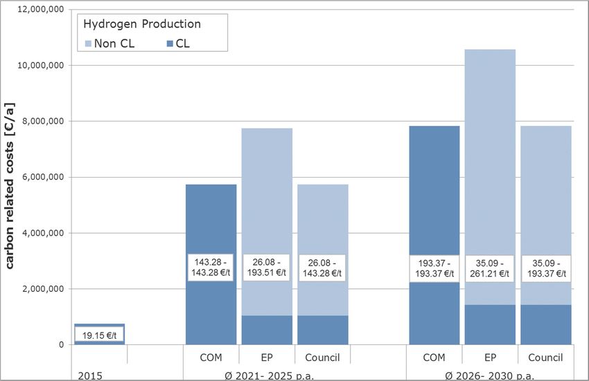
© FutureCamp Climate GmbH, 2017

FutureCamp Climate GmbH
Aschauer Str. 30
81549 München, Germany

www.futurecamp-climate.de
climate@future-camp.de
Tel +49 (89) 45 22 67 -0

This study has been conducted by
FutureCamp Climate GmbH
in cooperation with
FutureCamp Holding GmbH

FutureCamp
is a Munich based consultancy established in 2001 which provides strategic and
operational consulting services in the areas of climate, energy, and environment on the
national and international level.

VIK – Verband der Industriellen Energie- und Kraftwirtschaft
is the German Association of Industrial Energy Consumers which, as a cross-sectoral
organisation, represents the interests of and advises its member companies on all issues
related to energy economy and energy policies. Founded in 1947, VIK represents 80% of
the German industrial energy consumers and 90 % of the electricity producers that are
independent from utility firms. The products and services of its members are of great
importance for the value chains, climate change, and the German energy transition.

                                           2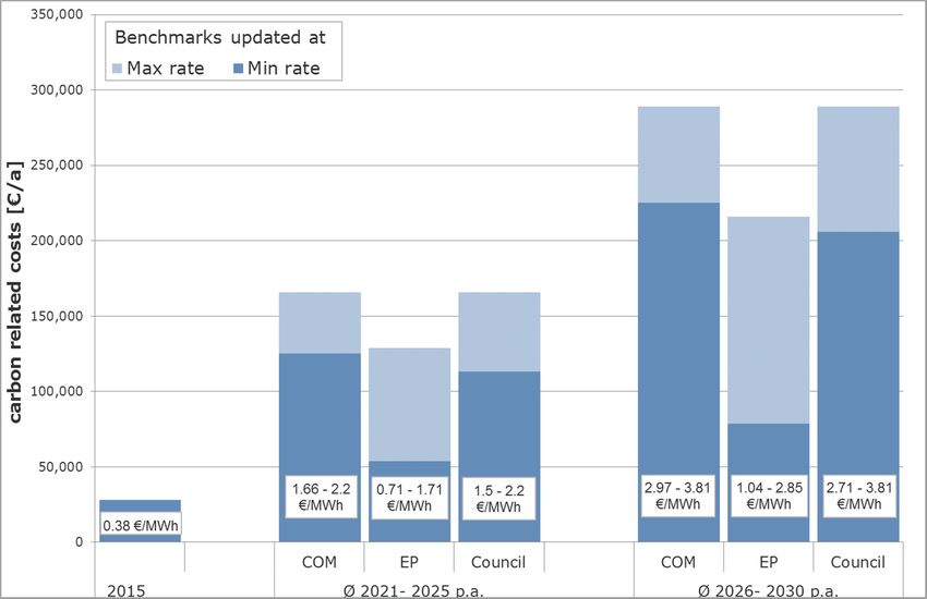
Table of contents
1   Summary ........................................................................................................... 4

2   Key Findings ....................................................................................................... 5

3   Introduction ........................................................................................................ 6

4   Results ............................................................................................................... 8
    4.1    EUA quantities ............................................................................................. 8
           4.1.1 Comparison of the EU ETS revision proposals ........................................ 8
           4.1.2 Cross-sectoral correction factor .......................................................... 10
    4.2    Case studies .............................................................................................. 12

5   Annex: Assumptions ........................................................................................... 20

Disclaimer

This study has been conducted with the greatest possible care. However, no warranty is
given as to the accuracy or completeness of the information contained in this publication.
This study was financed by VIK - Verband der Industriellen Energie- und Kraftwirtschaft
e. V. However, the results presented in it, the information contained in it, and the views
expressed are those of FutureCamp. They are not or not necessarily those of VIK and its
members.
Neither FutureCamp nor VIK adopt positions of single companies or other associations
with regard to the current debate about the revision of the European Union Emissions
Trading System (EU ETS) for the 2021-2030 period. Also, no conclusions regarding these
positions can be drawn from this study. This is in particular the case for the assumptions
on which the calculations are based.

                                                          3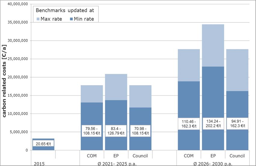
1 Summary
This study is based on the predecessor VIK study “The financial burden for Industry
arising from the revision of the EU ETS” conducted by FutureCamp in August 2016 which
compared carbon costs for industry on the basis of two scenarios: first, the EU
Commission’s proposal for the EU ETS revision submitted in July 2015 and, second, a
modified scenario which partly reflects VIK´s proposal for a dynamic EU ETS.
The aim of this follow-up study is to determine and present plant-specific CO2 costs
arising from the three proposals on the revision of the EU ETS issued by the European
Commission (COM), the European Parliament (EP), and the Council of the European
Union (Council). Based on these proposals the current trilogue takes place aiming at
finding an agreement on the future design of the fourth trading period of the EU ETS,
2021-2030.
The selected case studies represent sectors that are considered vulnerable to carbon
leakage.
Just like its predecessor, the follow-up study shows that carbon-related costs remain a
serious challenge for industry in the European Union (EU): They will rise significantly until
2030, creating very different situations for particular installations. The main drivers for
costs are carbon prices, benchmark updates, and the cost effect on the electricity price.
The application of a cross-sectoral correction factor (CSCF) could further increase the
financial burden.
Taking all three proposals for the revision of the EU ETS into consideration, the study
shows that the different numerical implications deriving from the proposals deserve a
closer look. This in-depth analysis allows to give recommendations on how the future EU
ETS should be designed.
The proposal of the EP with an optional 5% top-up offers the largest free allocation
budget. While in the understanding of FutureCamp the innovation fund is financed
through the auctioning share, the free allocation budget is partly used to fund the new
entrants reserve and the compensation of indirect costs of electricity prices. The Council
proposal offers the second largest budget for free allocation. It would be even more
effective in reducing the risk of carbon leakage (CL) if the free allocation budget was
further increased.
The flexibilities that have been proposed by the EP and the Council to avoid a CSCF help
reducing this risk significantly. However, the study shows that a CSCF is still not ruled
out completely. Whether it applies depends upon a number of choices regarding the
available budget, benchmark updates (real or flatrate), and other factors. The EP
proposal would apply the CSCF only to certain sectors (tiering) and could therefore lead
to deep cuts in free allocation for these sectors. To avoid a CSCF, the weighted average
benchmark update within the proposed budgets would need to be ca. 0.5 (Council), 0.6
(COM), or 0.35 (EP).
The case studies show that the update of benchmarks is an issue of high importance. The
updates of the fallback benchmarks, particularly for heat, have significant impacts on a
broad number of sectors. Equally important is the minimum update rate for benchmarks,
in particular for sectors that increasingly face physical and technological boundaries
raising their efficiency. Here, the proposals of the EP and the Council clearly better
address the needs of industry than the COM proposal.
Ensuring the carbon leakage status can be of vital importance for certain products or
sectors. As the examples of the iron and steel industry (for sinter) and of industrial gases
illustrate, this is not completely clear within the proposals at hand.
Also highly important is the compensation for indirect costs, as the example of the
aluminium industry shows. For many industries indirect costs are equally or even more
significant than direct costs. Therefore, it is essential to ensure that compensation of
these costs is not limited, but can be provided up to the level necessary.

                                             4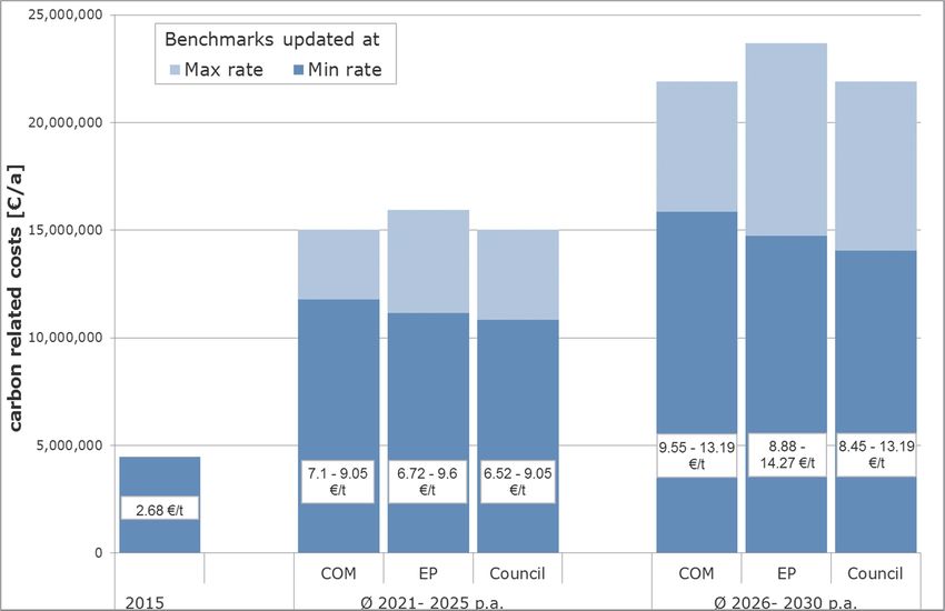
With calculations based on EU-wide European Union emission allowances (EUA) budgets
and unified rules and case studies conducted at installation level, the results do not
exclusively reflect installations in Germany but can be transferred to similar installations
in other EU member states.

2 Key Findings
There are two overarching findings that can be derived from the analysis of the positions
of the COM, EP, and the Council with regard to the effects on plant-related carbon costs:
   1. In all three proposals for the revision of the EU ETS, the financial burdens
      increase for the years 2021 to 2030.
   2. A rising carbon price is to be expected due to the reductions of the amount of
      allowances.
The findings of this study confirm the results derived from its predecessor study.

Furthermore, the following three cross-sectoral findings can be extrapolated:
   1. It is important to avoid a CSCF through an adequate extension of the budget for
      free allocation. Unlike the COM proposal, the free allocation budget suggested by
      the EP and the Council would allow moderate minimum benchmark update rates
      without triggering a CSCF.
   2. For several types of installations, state aid for indirect costs is crucial, and even
      more important than free allocation or direct carbon costs. The rules for future
      state aid still need to be finalised. It is essential that they are designed in a way
      that effectively reduces the risk of carbon leakage. If the degressive path is
      continued, as proposed by the EP, indirect costs will rise even more.
   3. The adjustment of the heat benchmark is a cross-cutting issue that could cause
      significant additional costs for a large number of sectors.

Finally, detailed sector-specific findings are included in the case studies.

                                              5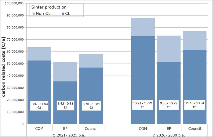
3 Introduction
Purpose
This study assesses the carbon-related costs that may result from different designs of the
EU ETS for the 2021-2030 timeframe1. The study focuses particularly on energy-intensive
industries in Europe. It assesses the costs that would potentially result from the
proposals for an EU ETS revision of the COM2, EP3, and the Council4.

Thematic areas
The study has two thematic areas: In the first part, EUA quantities for the different
positions have been calculated. This part also includes calculations of the CSCF. In the
second part, carbon-related costs for energy-intensive industries are determined at
installation level. Calculations have been performed for the following sectors and types of
installations:
      -    Chemical industry: Energy Production (steam)
      -    Chemical industry: Combined Heat and Power (CHP)
      -    Chemical industry: Steam Cracking
      -    Iron and steel: Steel Production
      -    Industrial gases: Steam Reforming
      -    Non-ferrous metals: Aluminium Electrolysis
The case studies illustrate different forms of cost impacts. They have been chosen to
analyse different aspects like e.g. the significance of the carbon leakage status for
particular sectors, the role of compensation for indirect costs, or the rules for updating
benchmarks. The selection of installations and sectors, however, does not indicate that
sectors or installation types that are not represented in the case study, e.g. the
production of paper, glass, cement are not affected in similar ways. The cases have been
selected to represent all relevant challenges and, at the same time, avoid repetitions.

Background
The results presented here are an update and further development to FutureCamp’s 2016
study for VIK.5 The following companies have taken part in the study and its 2016
predecessor:
      •    AIR LIQUIDE Deutschland GmbH
      •    BASF SE
      •    Covestro Deutschland AG
      •    Currenta GmbH & Co. OHG
      •    Evonik Industries AG
      •    Hydro Aluminium Rolled Products GmbH
      •    Ineos Köln GmbH

1
    Indirectly, the study also assesses indirect carbon-related costs. This requires assumptions for new State Aid
    Guidelines for indirect costs. These assumptions can be found in the annex.
2
    As communicated on 15 June 2015: COM(2015) 337.
3
    As agreed on 15 February 2017
4
    As agreed on 28 February 2017
5
     http://vik.de/pressemitteilung/items/vik-studie-zur-kostenbelastung-energieintensiver-industrien-durch-den-
    eu-emissionshandel.html

                                                         6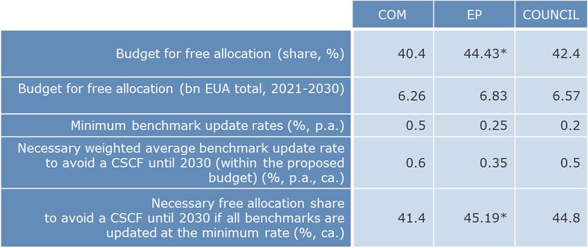
•    Linde AG
      •    SCA GmbH
      •    thyssenkrupp Steel Europe AG
      •    TRIMET Aluminium SE
      •    UPM GmbH

Approach
The quantification of the different positions of the EU institutions regarding the revision of
the EU ETS is based on a document analysis of the positions, empirical data, and
calculations by FutureCamp. The resulting quantities have been used to calculate the
CSCF for different scenarios. These calculations have been performed in a purpose-built
tool that is operated by FutureCamp. They are also based on assumptions for future
production volumes, specific CO2 emissions, and specific electricity demands.
The case studies are related to existing installations in Germany. To ensure anonymity,
data has been distorted. The only exceptions from this approach are the case studies for
the CHP plant and for the iron and steel sector. For the latter, the sector’s German
association6 has defined a virtual installation that represents a typical integrated plant.
The following table gives an overview of the most important assumptions of the study.

                                   Table 1: Key assumptions for the case studies.

While most assumptions are related to political choices, the carbon price is somewhat
different. It is an external variable that cannot be predicted within this study. Here, the
following approach has been chosen: To ensure consistency with the 2016 study, carbon
prices have not been changed. They start from actual levels in 2013 through 2015 and
then rise on a linear path up to 30 € in 2030. Compared to the 2016 study, the assumed
2030 price level of 30 €/EUA is regarded even more likely underlying the positions of the
EP and the Council. Especially the cancellation rule for EUAs in the Market Stability
Reserve (MSR) in the latter position is assumed to drive prices up as it delivers a political
signal that might influence expectations of market actors.
More information on methodology and assumptions is provided in the Annex.

6
    Wirtschaftsvereinigung Stahl

                                                         7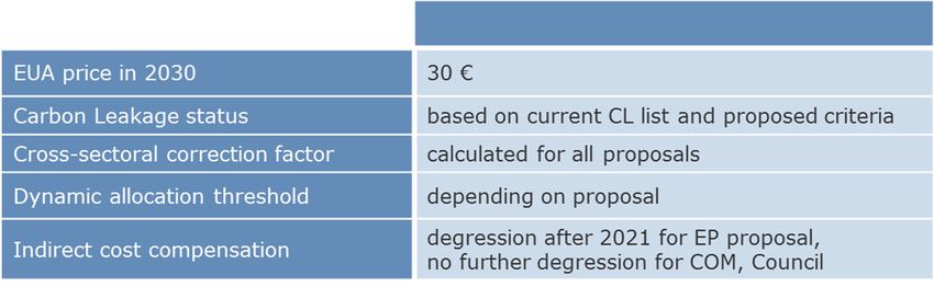
4 Results
4.1 EUA quantities
The three proposals provide different quantities of available EUAs for the 4th trading
period. In the following subsections, these quantities are discussed with regard to the
overall number of EUAs (Cap) and the respective budgets for free allocation in 2021-
2030.

4.1.1 Comparison of the EU ETS revision proposals

The EU ETS Cap
In 2013, the annual Cap was ca. 2.08bn EUA. In 2020, it will be 1.82bn EUA. For the
COM and Council positions, the 2030 Cap will be reduced to 1.33bn EUA. If the LRF is
increased from 2.2% p.a. to 2.4% p.a. in 2024 (EP7), the Cap in 2030 will be 1.30bn
EUA.
The total Cap for the 8 year timeframe from 2013-2020 is 15.60bn EUA. For the 10 years
period from 2021-2030, the total Cap will be 15.50bn EUA, if the LRF is 2.2% p.a.. If the
LRF would be raised to 2.4% p.a. in 2024, the total Cap will be reduced by 123m EUA to
15.38bn EUA.

                                      Figure 1: Comparison of Caps for EUA

7
    To adjust the LRF to 2.4% from 2024 is optional in the EP position. Here, it is assumed that the LRF will be
    increased from 2.2% p.a. to 2.4% p.a. in 2024.

                                                        8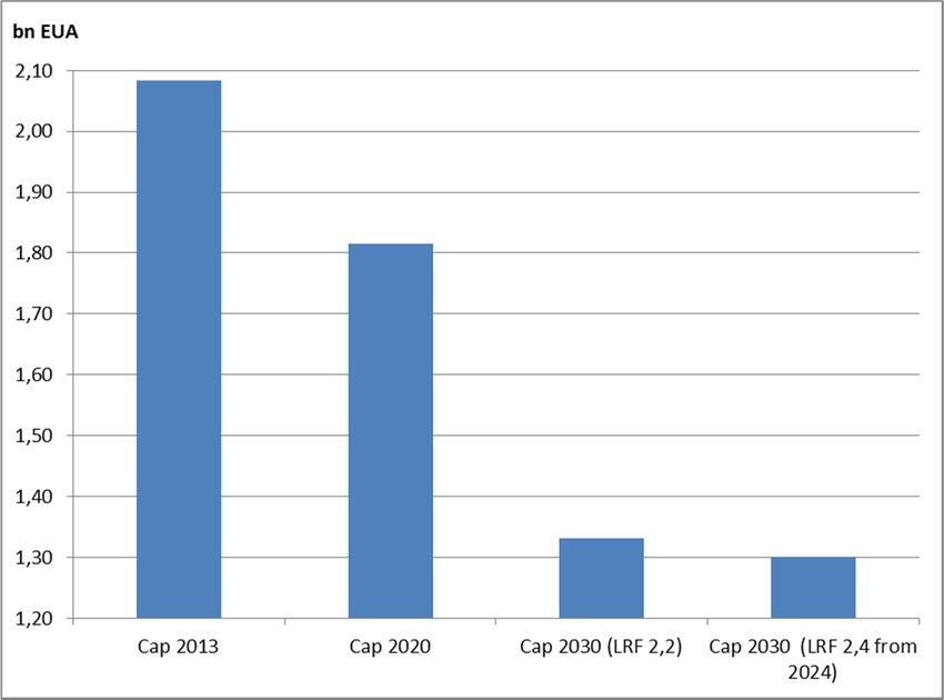
The budget for free allocation
The actual amount of certificates available for free allocation is different for all three
proposals.
In the COM proposal, a share of 40.4% of the Cap is available for free allocation. This
equals ca. 6.26bn EUA over the entire fourth trading period.
The EP position contains a provision that allows extending the budget for free allocation
by 5 percentage points of the Cap in order to avoid the application of the CSCF. However,
two reductions from the budget for free allocation have to be taken into consideration as
well:
        (1) 400m EUA for the new entrants reserve (NER) do not come from the third
trading period of the EU ETS8 and the market stability reserve (MSR), but from the free
allocation share 2021-30.9
       (2) 1% of the budget for free allocation is auctioned to fund compensation of
indirect costs. In the understanding of FutureCamp, the current EP position foresees the
600m EUA for the innovation fund to come from the auctioning share. In total, the
budget for free allocation adds up to ca. 6.83bn EUA over the entire fourth trading
period. The EP position therefore offers the largest budget for free allocation.
The Council position reserves additional 2 percentage points of the Cap for free allocation
in case a CSCF would apply. With no further reductions, the overall budget for free
allocation adds up to 6.57bn EUA over the entire fourth trading period.

                                      Figure 2: Overall free allocation budgets

8
    The third trading period is from 2013-2020.
9
    In the other positions, the certificates for the Innovation Fund come from the third trading period and are thus
    on top of the overall 2021-2030 cap.

                                                          9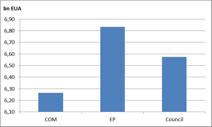
4.1.2 Cross-sectoral correction factor
A CSCF applies, if the volume of preliminary free allocation exceeds the available budget.
In contrast to the current third trading period, a number of flexibilities have been
proposed to the fourth trading period to limit the risk of a CSCF. In most scenarios a
CSCF does not apply. However, the complete prevention of a CSCF is not guaranteed.
The factors that determine the likelihood of a CSCF are the budget available for free
allocation and the factors to calculate preliminary free allocation, namely, production
levels, benchmarks, and carbon leakage status.
Calculations were carried out with the FutureCamp CSCF calculator. Key findings of these
calculations are:
- Benchmarks, carbon leakage rules, and the overall budget are the most important
factors with regard to design features. Among benchmarks, there are some major
ones that have a high impact on the result, like heat, grey cement clinker, hot
metal, refineries (complexity weighted tonne, CWT), and fuel. More than 70% of
free allocation is based on these five benchmarks. If all major benchmarks are
adjusted at their minimum rate, a CSCF applies for all three proposals (COM, EP,
Council), with the highest cuts through a (selective) CSCF under the EP proposal.
- Specific provisions (e.g. for particular benchmarks or the discontinuation of
applying the LRF for CHP as proposed by the EP) have additional impact on the
CSCF.
- If, depending on the particular proposal, the overall weighted average of
benchmark adjustment is between 0.35 and 0.6% p.a., a CSCF is not expected to
apply.
Likeliness of a CSCF in the different proposals
COM position: In the COM proposal, a CSCF is not expected. The most important factor
here is that the minimum update rate of 0.5% p.a. for benchmarks is the highest in all
three proposals. With a weighted average benchmark update of roughly 0.6%, no CSCF
would apply in this scenario.
EP position: In the EP scenario, it is unlikely that a CSCF applies. The minimum update
rate is 0.25%. With a weighted average benchmark update of 0.35%, no CSCF would
apply in this scenario. Nevertheless, it is important to note that due to a specific
provision, the CSCF would only apply for certain sectors and would effectively be much
stricter for them. Based on data from the current Carbon-Leakage list, among these
sectors would be cement, lime and plaster, bricks and tiles, and potentially industry
gases.
Council position: In the Council scenario, a CSCF might apply. The minimum update rate
is 0.2%. With a weighted average benchmark update of roughly 0.5%, no CSCF would
apply in this scenario. This, however, depends on the exact benchmark updates and it
should be noted that this study is not a benchmark study.
A CSCF could apply in modified scenarios. Two very prominent aspects of the EP position
that are not part of the Council position are the update of the hot metal benchmark and
the application of the CSCF instead of the LRF for some installations. If these options
were included in the Council scenario and particularly the budget in the Council scenario,
a CSCF of 0.96 would apply for 2026-2030 (with no CSCF before). Under this
assumption, a CSCF could most likely be avoided if an extra percentage point of the Cap
was used for free allocation.
It must be noted that there remain a number of relevant uncertainties:
This study is not a benchmark study and FutureCamp is well aware that in particular
the update of certain benchmarks has a significant influence on the CSCF. The most
important political choice is the update of the heat benchmark, the fuel benchmark,
10the inclusion of waste gases used for electricity production in benchmark calculation,
and the provision to apply the CSCF to a limited number of sectors (EP scenario).
The most influential general “unknowns” are future activity levels.
Furthermore, it should be noted that in order to assess the carbon leakage status of
all sectors and examples, the information included in the decision on the current CL
list10 is used. However, new data also might change the CL status of certain sectors
or sub-sectors.
Table 2: Free allocation share. *The free allocation share in the EP scenario relates to a budget that is
calculated based on the assumption that the LRF is adjusted to 2.4 in 2024
10
See http://eur-lex.europa.eu/legal-content/EN/ALL/?uri=CELEX:32014D0746
114.2 Case studies
Six cases have been analysed to better understand the impacts of the different proposals
for the future EU ETS design, and, furthermore, the design of the State Aid Guidelines.
The case studies refer to the installation level, not the sectoral level. This allows for a
precise analysis of impacts at installation level while some general conclusions can also
be drawn. With calculations based on EU-wide EUA budgets and unified rules and case
studies conducted at installation level, the results do not exclusively reflect installations
in Germany but can be transferred to similar installations in other EU member states.
The most significant results of the calculations by FutureCamp are summarized and
described in the subsequent tables and graphs. Each case study has a different focus,
depending on the particular challenge of each installation. The selection of installations
and sectors, however, does not indicate that sectors or installation types that are not
represented through a case study are not affected in similar ways.
In the case studies presented below, a CSCF of 1 is assumed for two reasons: Firstly, to
allow for the comparability of results and the isolation of relevant factors for specific
installations. The aspects that were analyzed in the case studies can be compared
between scenarios if the same CSCF assumption is underlying. Secondly, it is most likely
that no CSCF applies in the COM and the EP scenario11. In the Council scenario, a CSCF
might or might not apply after 2025, depending on the choices described above and
other factors, e.g. the assumed activity data. As the cases where a CSCF would apply
within the Council proposal require changes to the current proposal (e.g. by taking into
account the full carbon content of waste gases used for electricity production), it is
assumed that such changes could be linked with a slight increase in the budget.
Regarding the ambivalence of a CSCF application in the Council scenario and weighing it
with the methodological advantages described above, it seems reasonable to calculate
the case studies assuming that no CSCF would apply in the Council scenario, too.
However, FutureCamp is well aware, that the application of a CSCF cannot be ruled out
completely.
11
Plus, a CSCF in the EP scenario would not apply to the analyzed sectors due to the selective application of the
CSCF.
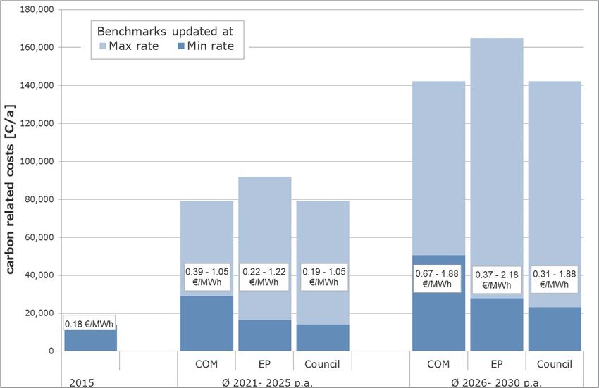
12Chemical Industry Energy Production (heat)
All parameters of relevance for free allocation applied here are assumptions. For example, the assumed
benchmark-update rate cannot be used to draw any conclusions on technological progress achieved or
expected for the (sub-)sector. Furthermore, the assumed increase of the price towards 30€/EUA in 2030
following a linear path is not a prognosis. All assumptions within this study do not allow to draw any
conclusion regarding the political positions of the companies participating or their industry associations.
Remarks:
The specific carbon costs in €/MWh relate to the product steam.
The case study is based on a natural gas fuelled installation which produces steam at an
efficiency close to the actual heat benchmark value. The steam is completely consumed
within installations that are exposed to a risk of carbon leakage (chemical sector).
The most relevant parameter influencing future carbon costs is the update rate of the
heat benchmark.
In the calculations, the CSCF of 1 is applied in all scenarios. The results show that
additional costs are in a similar range in all scenarios.
The state aid for indirect emission costs is not relevant in this case because heat is not
a product that is eligible for state aid according to the European guidelines on certain
state aid measures.
High update rates for the heat benchmark would lead to a large increase in carbon costs
even for an installation that is operated with natural gas close to the physical limit of
efficiency.
13Chemical Industry Energy Production (power and heat)
All parameters of relevance for free allocation applied here are assumptions. For example, the assumed
benchmark-update rate cannot be used to draw any conclusions on technological progress achieved or
expected for the (sub-)sector. Furthermore, the assumed increase of the price towards 30€/EUA in 2030
following a linear path is not a prognosis. All assumptions within this study do not allow to draw any
conclusion regarding the political positions of the companies participating or their industry associations.
Remarks:
The specific carbon costs in €/MWh relate to the product steam.
The case study is based on a natural gas fuelled installation which produces steam at an
efficiency close to the actual heat benchmark value. To an extent of 10%, there is also
generation of electricity within the installation and, therefore, the installation is
categorized as electricity producer. The steam is completely consumed within
installations that are exposed to a risk of carbon leakage (chemical sector).
The most relevant parameters influencing future carbon costs are:
update rate of heat benchmark
application of LRF or CSCF for electricity producers
In our calculations the LRF is applied in the COM and Council scenarios but in the EP
scenario no LRF is applied12. The results show that additional costs related to the
application of the LRF are significantly higher in the COM and Council scenarios than in
the EP scenario. Indirect costs and state aid are not considered here as the case study
focuses on an energy producing installation. However, indirect emission costs might
arise for installations consuming the electricity produced by the CHP.
The results show that the application of the LRF for electricity producers and high
update rates for the heat benchmark would lead to a large increase in carbon costs
even for an installation that is operated with natural gas close to the physical limit of
efficiency.
12
see amendment 70 in the EP position
14Iron & Steel Virtual Integrated Steel Plant All parameters of relevance for free allocation applied here are assumptions. For example, the assumed benchmark-update rate cannot be used to draw any conclusions on technological progress achieved or expected for the (sub-)sector. Furthermore, the assumed increase of the price towards 30€/EUA in 2030 following a linear path is not a prognosis. All assumptions within this study do not allow to draw any conclusion regarding the political positions of the companies participating or their industry associations. Remarks: Specific carbon costs are quantified in €/t of raw steel. The case study is based on a virtual integrated steel plant reflecting the average of European installations. As the case study is based on a virtual installation, no calculations are performed for actual years. The virtual plant produces electricity by itself mainly using waste gases as fuel (Blast Furnace Gas 70-80%, Coke Oven Gas 20- 30%, Natural Gas
metal14 in that scenario.
At the same time, the volume of electricity produced, which is not rewarded within
the compensation scheme for indirect costs, is 75% and reflects the average share
of waste gas used for electricity production that receives free allocation within the
hot metal benchmark. Thus, double counting through free allocation within the ETS
scheme and through state aid for indirect emissions costs is excluded.
State aid is reduced on a diminishing scale starting from 0.7% in 2021 (0.7) and
resulting in 0.6% in 2030.
The reassessment of the hot metal benchmark is the most relevant factor influencing
the carbon costs when comparing proposals, as the significantly lower costs in the EP
scenario show.
The second relevant issue is whether or not sinter is considered a carbon leakage
exposed sector. In the EP scenario, the consequences are even more severe as there
would be no free allocation for non-CL sub-installations at all.
The third relevant issue are the diverging minimum rates for benchmark updates.
Comparing the results of the COM and the Council scenarios, the minimum update rates
range from 0.5 to 0.2% p.a..
14
http://www.eurofer.org/News%26Events/Archives/Press%20releases/EUROFER%20Goes%20to%20Court%20
on%20EU%20ETS.fhtml
16Chemical Industry Steam Cracking
All parameters of relevance for free allocation applied here are assumptions. For example, the assumed
benchmark-update rate cannot be used to draw any conclusions on technological progress achieved or
expected for the (sub-)sector. Furthermore, the assumed increase of the price towards 30€/EUA in 2030
following a linear path is not a prognosis. All assumptions within this study do not allow to draw any
conclusion regarding the political positions of the companies participating or their industry associations.
Remarks:
The specific carbon costs in €/t relate to the product „steam cracking (high value
chemicals)” as defined for the corresponding product benchmark.
The calculation results do not vary significantly among the positions. The most relevant
parameter influencing carbon costs is the update rate of the benchmarks. In case the
real improvement lies within the range of 0.5% p.a. and 1.5% p.a., the results are
similar for all three positions. In the EP scenario, state aid for indirect CO2 costs is
subject to further degression starting from 0.7% in 2021 and resulting in 0.6% in 2030.
17Industrial Gases Steam Reforming
All parameters of relevance for free allocation applied here are assumptions. For example, the assumed
benchmark-update rate cannot be used to draw any conclusions on technological progress achieved or
expected for the (sub-)sector. Furthermore, the assumed increase of the price towards 30€/EUA in 2030
following a linear path is not a prognosis. All assumptions within this study do not allow to draw any
conclusion regarding the political positions of the companies participating or their industry associations
Remarks:
The specific carbon costs in €/t relate to the product hydrogen as defined for the
corresponding product benchmark. The case study is based on a steam reformer
producing predominantly hydrogen.
Carbon-related costs for production of hydrogen (and its by-product syngas) are
particularly influenced by the question whether industrial gases will remain on the list of
sectors exposed to the risk of carbon leakage. So far, neither the position of the COM nor
the positions of the EP and the Council provide sufficient certainty that industrial gases
will be able to meet the relevant thresholds on sector or subsector level.
This is of particular importance since hydrogen and syngas can also be produced by the
refining and the chemicals sectors but in practice are very often outsourced to specialized
industrial gas producers for economic and ecological benefits. Therefore, any inconsistent
treatment of the identical production activity among those sectors would lead to severe
market distortions – particularly for the outsourced producers. Accordingly, both the EP
position and the Council position, include recitals indicating the need to harmonize not
only benchmark updates but also the determination of the CL status between the sectors
refineries and chemical industries15. However, it is not clear whether the recitals will be
sufficient to maintain the level playing field between insourced and outsourced producers
of hydrogen and syngas from the operator´s point of view.
Here, we do not assume a possible selective CSCF simply because the worst case under
the EP proposal for this activity might lead to a CL factor of 0. In this case, a (selective)
CSCF that might be applicable under the EP proposal would not lead to any additional
cuts for this installation.
15
see amendment 12 in the EP position
18Non-Ferrous Metals Aluminium Electrolysis
All parameters of relevance for free allocation applied here are assumptions. For example, the assumed
benchmark-update rate cannot be used to draw any conclusions on technological progress achieved or expected
for the (sub-)sector. Furthermore, the assumed increase of the price towards 30€/EUA in 2030 following a linear
path is not a prognosis. All assumptions within this study do not allow to draw any conclusion regarding the
political positions of the companies participating or their industry associations.
Remarks:
The specific carbon costs in €/t relate to the product aluminium as defined for the
corresponding product benchmark. More than 90% of the carbon related costs are indirect
ones. In the case of aluminium, it is possible to compare these costs with the market price
for aluminium set at the London Metal Exchange (LME). LME Cash Settlement Price is the
global reference price for aluminium and its average within the last 2 years was USD
1637.60 per ton (23 March 2015 through 22 March 2017). Using the exchange rate as of
23 March 2017 this means 1515.00 €/t aluminium. This means that e.g. for 2021-25,
carbon costs including the assumed compensation for indirect costs amount to roughly
4.7% of sales price in the assumed best case and 8.4% in the assumed worst case. For
2026-2030, these relations will rise up to 6.3% and 13.3% respectively.
The most relevant issue for this case study is the question of how compensation of indirect
costs will be designed in the future. The calculation results here are based on the
assumption that the general principles for the compensation of indirect costs that are
currently in place will also be used for 2021-2030. It is assumed that the relevant product
benchmarks will be updated to a similar extent as proposed for free allocation using the
same min/max values. Therefore, the update rates also have significant influence on the
results of this case study. Furthermore, consistency in state aid volumes is extremely
important in this case. The same value as defined for 2020 (0.75) is assumed for the COM
and the Council, although both have not mentioned state aid intensity and development. In
contrast, the EP position explicitly foresees a continuation of degression. In the EP scenario
the volume of state aid, thus, is reduced on a diminishing scale starting from 0.7% in 2021
to 0.6% in 2030.
Another assumption is that compensation will not be subject to any reduction factors
deriving from a defined overall limit on compensation payments (e.g. expressed as
percentage of auctioning revenues). If this was the case and applied here, indirect costs
would increase even more depending on the additional reduction factor.
195 Annex: Assumptions
The case studies have been carried out based on the following assumptions:
Carbon price Starting with empirical values for 2013-2015. Linear increase up
to 30 €/EUA in 2030
2021-2025 average: 19.94 €/EUA
2026-2030 average: 27.13 €/EUA
Carbon leakage exposure factors 1 for CL sectors (all proposals)
0.3 for non-CL sectors (COM, Council)
0 for non-CL sectors (EP)
Cross-sectoral corrector factor CSCF = 1 for all scenarios
Linear reduction factor COM, Council: LRF = 2.2
EP: LRF = 2.2; from 2024: 2.4
Benchmark updates (% p.a.) 0.5/1/1.5 (COM)
0.25-1.75 (EP)
0.2-1.5 (Council)
Dynamic allocation threshold 10% (EP)
15% (Council)
50% (COM)
Assumptions for indirect carbon costs Grid emission factor: 0.76 tCO2/MWh
Volume of state aid:
- Council, COM : 0.75 (assumption; COM and Council
proposals have not discussed state aid intensity and
development since this is left to DG Comp)
- EP: 0.7 (2021-2023), 0.65 (2024-2026), 0.6 (2027-2030)
Sector-specific assumptions for future development of production
levels, specific emissions, and specific electricity demand.
To calculate direct and indirect carbon- Free allocation
related costs, participating companies Emissions
have provided the following data for the
years 2013-2015 Production levels for all sub-installations
Production levels relevant for indirect costs
Substitution factors (fuel-electricity) if relevant for the respective
product benchmark
Total electricity consumption (from grid and self-generated
[covered by the ETS])
Compensation for indirect CO2 costs
Calculations for the 2016-2030 timeframe have been performed on the basis of real data.
Depending on the available data, different forecasting methods were used:
„Input data“: individual forecasts for the operator until 2030.
„Linear specifications“: a linear development from 2013-2015 average values was
assumed
„Fluctuating specifications“: forecasts take the fluctuating pattern of the 2013-2015
timeframe into account. This modification has been defined to understand the effects
of dynamic allocation. This would not be possible on the basis of linear growth.
The calculation of free allocation was based on the following methodology:
2013-2020:
- Option 1: data according to the notification on free allocation
- Option 2: “adjusted base period“: calculations on the basis of actual activity levels
for the respective years. Adjusted by variations in production since the base
period of the actual trading period
20 2021-2025: calculation depending on the dynamic allocation threshold
- If the activity level variation is below the threshold: calculation based on the
median of activity levels 2013-2017
- If the activity level variation is above the threshold: calculation based on the
activity levels in the actual year
- Definition of „dynamic allocation threshold“: change of activity levels in the
reporting year compared to the 2013-2017 median
2026-2030: calculation depending on the dynamic allocation threshold
- If the activity level variation is below the threshold: calculation based on the
median of activity levels 2018-2022
- If the activity level variation is above the threshold: calculation based on the
activity levels in the actual year
- Definition of „dynamic allocation threshold“: change of activity levels in the
reporting year compared to the 2018-2022 median
For all cases, free allocation and direct carbon-related costs16 have been calculated. The
ratio of both expresses (in percent) the degree to which an operator is equipped with
EUAs compared to his emissions. Using this value, real direct carbon-related costs have
been calculated and expressed as absolute values and as specific values per unit of
product.
Calculation of the compensation for indirect carbon costs were based on the following
methodology:
2013-2020:
- Calculation based on activity rate in the respective year
- Plausibility check through comparison with real 2013/2014 data
- For methodical reasons, no limitation of compensation volumes was assumed
2021-2030:
- Calculation based on activity rate in the respective year
- For methodical reasons, no limitation of compensation volumes was assumed
For all cases with indirect costs, the volume of state aid and indirect carbon-related costs
have been calculated. The ratio of both expresses the level of compensation of indirect
carbon costs. Using this value, real indirect carbon-related costs have been calculated
and expressed as absolute values and as specific values per unit of product.
16
Emissions multiplied with the actual EUA price.
21You can also read