POISSON TOTAL VARIATION DENOISING FOR MICROPULSE WATER
←
→
Page content transcription
If your browser does not render page correctly, please read the page content below
EPJ Web Conferences 237, 06012 (2020) https://doi.org/10.1051/epjconf/202023706012
ILRC 29

 POISSON TOTAL VARIATION DENOISING FOR MICROPULSE WATER
 VAPOR DIAL
 Matthew Hayman1, Willem Marais2, Robert Stillwell1, Scott Spuler1
 1National Center for Atmospheric Research, Earth Observing Lab, Boulder, CO 80303, USA
 2Cooperative Institute for Meteorological Satellite Studies, University of Wisconsin-Madison, USA
 *Email: mhayman@ucar.edu
 ABSTRACT Poisson Total Variation is a processing technique
 We have adapted the Poisson Total Variation lidar recently developed at University of Wisconsin for
 signal processing technique for Micro-Pulse DIAL high spectral resolution lidar (HSRL) retrievals and
 water vapor estimates. This processing technique has been shown to significantly improve extinction
 ingests data at 10 second-37.5 meter resolution and lidar ratio estimates from the UW HSRL
 where it adaptively adjusts the retrieval resolution instrument [5]. The technique leverages numerical
 based on signal-to-noise and performs range methods developed for Poisson image denoising
 deconvolution. The result is high resolution data in and deblurring [6,7]. PTV assumes that the
 regions with ample signal, preservation of sharp estimated lidar data products can be approximated
 discontinuities where they exist, and a data product by a linear piecewise function and effectively
 that better represents of the acquired photon adapts the region of estimation based on signal-to-
 counting data than the standard processing noise. It leverages correlations in the observed
 technique. image (in the case of lidar a time/range curtain) to
 infer the data product from the random noise
 without forcing the underlying signal to be band
 1. INTRODUCTION limited.
 Water vapor DIAL uses two closely spaced In a collaboration between NCAR and University
 wavelength, one tuned to a water absorption feature of Wisconsin, we have demonstrated the PTV
 (online) and a second tuned off the feature (offline) technique can be adapted for MPD water vapor
 to estimate range resolved water vapor estimates. While the approach is still under
 concentration in the atmosphere [1]. Through development, it shows promise for improving the
 knowledge of the water vapor absorption cross instrument’s capabilities by providing flexibility to
 section, the two observations can be directly related capture variations at higher resolution and
 to the water vapor number concentration. The increasing retrieval accuracy.
 power of this approach is that it requires no
 ancillary observations of atmospheric state for
 processing or calibration, making it a truly 2. METHODOLOGY
 independent of other water vapor observations. The PTV method for HSRL is detailed in [5], and
 In a collaboration between the National Center for the technique was adapted for processing DIAL
 Atmospheric Research (NCAR) and Montana State signals without sacrificing the advantages of the
 University, a Micro-Pulse DIAL (MPD) has been conventional DIAL technique. Specifically, it
 developed based on diode laser technology for allows estimation of water vapor without direct
 remote unattended operations over long periods of knowledge of the atmospheric aerosol loading,
 time [2,3,4]. The instrument lasers are invisible instrument effects common to both wavelengths
 and eye-safe and the receiver employs narrowband (e.g. geometric overlap) or scalar differences
 filtering and photon counting to observe weak between the two wavelength channels.
 signals day and night in clear and cloudy conditions. PTV requires a forward model to evaluate retrieved
 In order to obtain useful water vapor estimates, the parameters against raw photon counts. To
 standard MPD signal processing employs fixed implement this we add a second parameter retrieval.
 temporal smoothing between 1 and 5 minutes and The forward model consists of a profile that is
 range smoothing between 150 and 750 m dependent on the wavelength ( ), the water vapor
 (depending on signal-to-noise).

 © The Authors, published by EDP Sciences. This is an open access article distributed under the terms of the Creative Commons Attribution License 4.0
 (http://creativecommons.org/licenses/by/4.0/).
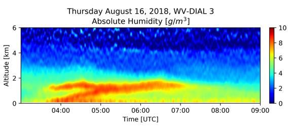
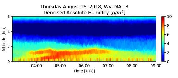
EPJ Web Conferences 237, 06012 (2020) https://doi.org/10.1051/epjconf/202023706012
ILRC 29

 density ( ) and a term that represents all terms that 3. RESULTS
 are common multipliers between the two Figure 1 shows an example of MPD retrievals
 wavelength channels ( ). The observed photon applied to data from August 16, 2018. The top
 counts at bin i and operational wavelength is panel shows our standard water vapor processing
 given by routine. The middle panel shows the water vapor
 estimate from the PTV processing method
 ( ) = ( ) (−2Δ ∑ ( ) ) + described here and the bottom panel shows the
 common terms obtained through the PTV method.
 =1

 Where ( ) is a constant multiplier specific to the
 laser wavelength of operation, ( ) is the water
 vapor absorption cross section at that wavelength,
 Δ is the range between data points and is the
 background.
 In principle, the common term can be estimated
 using a conventional DIAL processing approach,
 but it is not necessary and provides limited
 scientific value. For this analysis, we require
 estimating to forward model the retrieval and
 evaluate its accuracy.
 In our retrieval we allow the estimator to adjust the
 scalar gain of each channel ( ). Like , this falls
 out in standard DIAL processing but is needed for
 forward modeling. It has no impact on the actual
 water vapor estimate.
 The forward modeled profiles are evaluated using
 the inverse log-likelihood for a Poission
 distribution. Lower values of this function
 indicate a better fit. We also include a regularizer
 term to penalize variation in the retrieved profile.
 The overall minimization is performed on

 ( , ) = ∑ ∑ ( ) − ( ) ln ( ) Figure 1: Water vapor estimates from an MPD using the
 =1 standard inversion (top) and PTV inversion (middle).
 + ‖ ‖ + ‖ ‖ For context, the PTV estimated common terms are
 shown (bottom).
 such that the solution is
 We note that there are some key differences
 , ( , ), between the standard and PTV processing
 techniques. First the PTV method captures sharper
 where the forward model ( ) is a function of the discontinuities in the water vapor profile because
 water vapor density ( ) and multiplier term ( ). PTV approximates the water vapor field as a linear
 The term ‖ ‖ evaluates the sum of the absolute piecewise function. This is in contrast to the our
 value of all changes in in both time and range and standard Savitzky-Golay filtering and Gaussian
 and are regularization coefficients that smoothing approach used in the top panel, which
 determine the amount of penalty imposed for effectively limits the sharpness of the profile.
 variation in the estimated water vapor and common
 In the region above 3 km, the PTV better captures
 terms.
 the dryness of the air by using larger pieces, while

 2
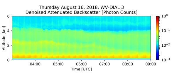
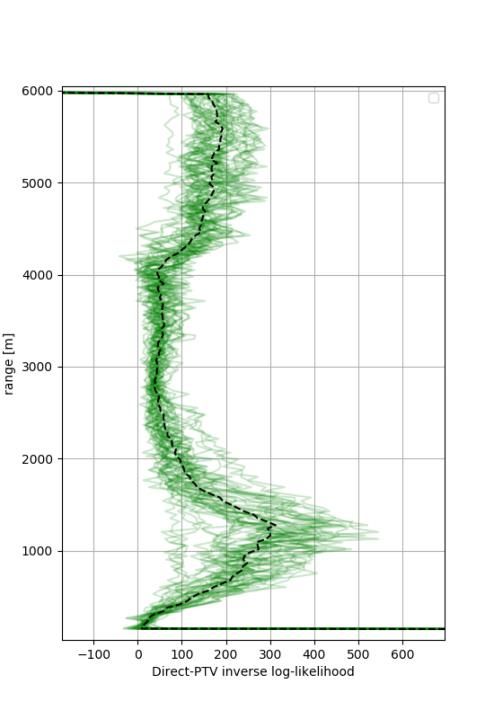
EPJ Web Conferences 237, 06012 (2020) https://doi.org/10.1051/epjconf/202023706012
ILRC 29

 the standard processing approach has substantial observation that is statistically independent from
 noise that deceptively looks like enhanced water (a the original retrieval data. These separate retrieval
 product of the color scale having a minimum value and verification datasets are obtained from a single
 of zero). photon counting MPD profile using Poisson
 thinning, where the underlying signals are common
 The PTV estimate shows an artificially high water
 to both datasets, but their Poisson noise is
 vapor content at the top of the profile above 5.5 km.
 statistically independent. We forward model the
 We suspect this artificially high region is the result
 two water vapor estimation approaches using the
 of low signal, where the optimizer did not adjust
 common terms from the PTV method in both cases.
 the water vapor estimate because it had little impact
 We found using the standard approach to estimate
 on the forward model error.
 made its forward model evaluate worse and we
 The PTV method also appears to be having do not want to penalize the approach for a
 problems estimating water vapor in the lowest secondary, typically unused, parameter. The
 range bins below 500 m where there is significant difference in the inverse log-likelihoods are shown
 striping throughout the time series. This may be in Figure 2, where positive values indicate better
 the result of the outgoing laser shot contaminating agreement from PTV water vapor estimates and
 the return signal. We note that the standard method negative indicates better agreement from the
 also appears to have problems in this region, standard approach.
 though they are less severe.
 From Figure 2, it is clear that the PTV method
 provides a better overall reflection of the lidar
 profiles. The preservation of higher frequency
 structure seems to improve the forward signal
 reconstruction below 2 km and above 4 km.
 Notably the artificially high water vapor does not
 seem to have a significant impact on the
 verification process, again suggesting that there is
 not enough information content in this region (i.e.
 there is high signal uncertainty) to estimate water
 vapor concentration.

 3. CONCLUSIONS
 The PTV signal processing method appears to be
 promising, for developing high accuracy water
 vapor estimates from photon counting MPD.
 However there are practical challenges to the
 technique. Signal processing is computationally
 expensive. The data set shown here was processed
 on a desktop computer and took approximately one
 day to complete. At present, there is no fast way to
 Figure 2: Difference in inverse log-likelihood between estimate uncertainty in the retrievals. Current
 direct water vapor inversion and PTV inversion for the techniques employed for HSRL retrievals employ
 vertical profiles in Figure 1. The median is indicated by ensemble approaches with various initial
 the dashed black line. Positive values indicate better conditions making the computationally expensive
 validation in the PTV retrieval. though parallelizable.
 To analytically assess the two retrieval methods we Never-the-less these issues are not necessarily
 use the inverse log-likelihood ( , ),without the major limitations. Advances in and availability of
 regularizer term where we compare the forward high speed computing resources continue to
 modeled retrievals against a verification improve. There is currently work to implement

 3
EPJ Web Conferences 237, 06012 (2020) https://doi.org/10.1051/epjconf/202023706012
ILRC 29

 PTV on GPUs and we continue to pursue
 opportunities to develop faster uncertainty
 estimates.

 ACKNOWLEDGEMENTS
 The National Center for Atmospheric Research is
 sponsored by the National Science Foundation.

 REFERENCES
 [1] Schotland, R. M. “Some observations of the vertical
 profile of water vapor by means of a laser optical
 radar,” in 4th Symposium on Remote Sensing of the
 Environment, (Michigan, 1964).
 [2] Nehrir, A. R., et al., ”Water vapor profiling using a
 widely tunable, amplified diode-laser-based
 differential absorption lidar (DIAL),” J. Atmos.
 Ocean. Technol., 26, pp. 733–745,
 doi:10.1175/2008JTECHA1201.1 (2009).
 [3] Spuler, S. M., et al., ”Field-deployable diode-
 laserbased differential absorption lidar (DIAL) for
 profiling water vapor,” Atmps. Meas. Tech, 8, pp.
 1073–1087, doi:10.5194/amt-8-1073-2015 (2015).
 [4] Weckwerth, T. M., et al., “Validation of a Water
 Vapor Micropulse Differential Absorption Lidar
 (DIAL),” J. Atmos. Ocean. Technol., 33, pp. 2353–
 2372, doi: 10.1175/JTECH-D-16-0119.1 (2016).
 [5] Marais, W. J., et al., “Approach to simultaneously
 denoise and invert backscatter and extinction from
 photon-limited atmospheric lidar observations,”
 Appl. Opt., 55, pp. 8316-8334,
 doi:10.1364/AO.55.008316 (2016)
 [6] Wright, S., et al., “Sparse reconstruction by
 separable approximation,” IEEE Trans. On Signal
 Proc., 57, pp. 2479-2493 (2009),
 doi:10.1109/TSP.2009.2016892.
 [7] Harmany, Z. and R. M. Willett, “This is SPIRAL-
 TAP: Sparse poisson intensity reconstruction
 algorithms-theory and practice,” IEEE Trans. On
 Image Proc., 21, pp. 1084-1096,
 doi:10.1109/TIP.2011.2168410 (2012).

 4
You can also read