Predicting the development of the NBA playoffs.
←
→
Page content transcription
If your browser does not render page correctly, please read the page content below
VRIJE UNIVERSITEIT AMSTERDAM

Predicting the development
of the NBA playoffs.
How much the regular season tells us about the playoff
results.

Max van Roon
29-10-2012

Vrije Universiteit Amsterdam
Faculteit der Exacte Wetenschappen
Studierichting Business analytics
De Boelelaan 1081a
1081 HV Amsterdam

Supervisor: dr. Z. Szlavik
PREFACE

During the Business Analytics master, each student has to produce a paper about a research the
student has done. This research can be about a subject of the students choice, but has to include
some components from the Business Analytics courses.

This paper will be about the study I have done on the NBA playoffs. The main goal during the
study was to build a model which predicts the development of the NBA playoffs, given the data
which is available beforehand. This means the data from the regular season will be used to
predict the playoffs.

During this study I especially used the skills I learned from dr. Z. Szlavik, during the course Data
Mining Techniques. More thanks to dr. Z. Szlavik for supervising this research.

2
ABSTRACT

Each year, after the regular season, the NBA playoffs are played to determine the NBA champion.
The main goal of this research was to build a model which predicts how the NBA playoffs will
develop. For each round the winners will be determined. This is done by predicting all possible
games to be played in the best-of-seven series. This means all possible combinations of scores at
home- and away-games. The model gives a probability for each score and thereby a probability
for each team to compete in the playoffs. Performance is measured by probabilities assigned to
the competing teams and by percentage of right predicted competing teams. For modeling, three
algorithms are chosen: naïve bayes, decision tree and k-nearest neighbors. As attributes the
team seedings, winning percentages and several season statistics were used. The models are
trained and tested on the last 9 seasons. Training is done on eight years, and the model is tested
on the other one. Two models have been found. The model which performed best on probability
used the k-nn algorithm. The average probability assigned to the competing teams was 75%. The
model which performed best in just choosing the winner used the naïve bayes algorithm and
performed 77%.

3
CONTENTS
Preface ...............................................................................................................................................2
Abstract ..............................................................................................................................................3
Introduction........................................................................................................................................6
1.     Previous Research .......................................................................................................................7
       1.1 Previous Research .................................................................................................................7
       1.2 Compared to this research ....................................................................................................8
2.     Methods .....................................................................................................................................9
       2.1 Collecting the data ................................................................................................................9
       2.2 Building the model ................................................................................................................9
3.     Attributes.................................................................................................................................. 11
       3.1 Team ................................................................................................................................... 11
       3.2 Playoffs ............................................................................................................................... 11
       3.3 Seasons statistics ................................................................................................................. 12
4.     Data Analysis............................................................................................................................. 13
       4.1 NBA Season ......................................................................................................................... 13
       4.2 Single games ....................................................................................................................... 13
       4.3 Best-of-7 series.................................................................................................................... 14
5.     Algorithms ................................................................................................................................ 16
       5.1 Naïve Bayes ......................................................................................................................... 16
       5.2 Decision tree ....................................................................................................................... 16
       5.3 K-nearest neighbour ............................................................................................................ 16
6.     Results ...................................................................................................................................... 17
       6.1 Example .............................................................................................................................. 17
       6.2 First combinations ............................................................................................................... 18
       6.3 Further investigation ........................................................................................................... 21
       6.4 Algorithms........................................................................................................................... 22
7.     Final models.............................................................................................................................. 23
       7.1 Probability based................................................................................................................. 23
       7.2 Binomial based .................................................................................................................... 23
8.     Conclusions and Discussions...................................................................................................... 24
       the models ................................................................................................................................ 24
       the performance ....................................................................................................................... 24
       Discussion ................................................................................................................................. 24

4
Appendix I NBA 2012 ........................................................................................................................ 25 5
INTRODUCTION

After 82 games the regular NBA season is over. Though, for the 8 best performing teams from
each of the two conferences it is only just beginning. The playoffs, a best-of-seven elimination
tournament, will determine which team earns the NBA championship title. Millions of fans
around the world are anxious to know how the playoffs will develop.

Last nine years the NBA has had six different champions. 1 Each NBA-team has reached the
playoffs at least once and 16 out of 31 teams at least once reached the conference finals. These
results show the change in teams strength over the years. Because of this change it will be
impossible to predict the NBA winners of coming years, based on last year’s winners.
Fortunately, before the playoffs are played, there is a long regular season, in which every team
competes against every other to earn a place in the playoffs. This regular season provides us
with multiple statistics which might give some information and make it possible to simulate the
playoffs. An interesting element might be the home advantage or the percentage of games won
during the regular season. Using this information as attributes for a model makes it possible to
say something about the outcomes of the playoffs, based on the regular season.

Statistics from the regular season will be linked with the teams in the last 9 years of playoffs. The
data from these NBA playoffs will be used to build a model using datamining and machine
learning techniques. The playoffs will be simulated by this model.

Although there is a considerable ‘luck’ factor in sports, I expect it is possible to give a good
prediction based on data. In the papers, experts predict all basketball games . Loeffelholz
(Bernard Loeffelholz, 2009) has found these experts to predict 68,67% correct. Because the
predictions will not be done per game but per best-of-seven series, this study is expected to
perform better and thereby reach a performance of at least 68,67%.

1   Information about NBA has been found on the NBA website, www.NBA.com.

6
1. PREVIOUS RESEARCH

1.1 PREVIOUS RESEARCH
Several researches have been done to predict the results of the National Basketball Association.
Students from Cernegie Mellon University (Jackie B. Yang, 2012) used support vector machines
that made use of the kernel functions. Their model did not perform well on the attributes they
used. The students started with 14 attributes per team but they did not investigated the
possibility that using all of these attributes might lead to overfitting. This might be the case in
this research looking at the performance of 55%. In 55% of 30 actual played games, the winner
was correctly predicted.

Wei (Wei, 2012) has examined the use of naive Bayes. Wei used home and away winning rates.
While Jones (Jones, 2007) showed the existence of the home advantage, using this home and
away winning rates did not influence Wei’s predictions. The predictions performed even worse
while accounting for the seasons home/away records. This might indicate the playoffs home
advantage being really different from the seasons home advantage. While the best performing
team gets the home advantage it is interesting to find out whether the best teams wins because
of the home advantage or because they are simply the better team.

Loeffelholz (Bernard Loeffelholz, 2009) has predicted the playoffs using an extensive database,
not only containing team- but also player-statistics. Though I cannot get access to such an
extensive database, it is interesting to take a look at the results he achieved, how he did this and
what performance he achieved. A nice way dealing with such an extensive database are neural
networks. The idea behind a Neural Network is a hidden layer where the parameters change
while more data passes through. This way the algorithm ’learns’ while processing. This
algorithm takes some more time compared to, for example, the naive bayes. The performance is
usually higher, also shown by Loeffelholz. Three of his neural network algorithms outperform
the experts, performing on average 73%.

Predictions have also been done in other sports tournaments. For example in rugby (Cooper,
2011), where the chances are calculated for New-Zealand winning the Rugby World Cup. Instead
of predicting one winner, Cooper gave the chances of each team winning the tournament. Cooper
did not predict who would win the quarterfinals and then predict the semi-finals given these
winners. He predicted every teams chances of competing to the next round and then did the
same for all possible semi-finals. The different probabilities multiplied by each other gave him
the chances of each team winning the finals. This is an interesting way of dealing with the
problem of not knowing the semi-finals and the finals before the tournament starts.

7
1.2 COMPARED TO THIS RESEARCH
In the last part, several percentages are mentioned. Though these percentages give us some
information about the predictability of the playoffs, they cannot directly be used in the upcoming
research. The 55% performance of the first research is based on a comparable dataset. This
55% seems very low for predicting results of playoff series. Playoff series seem to be quite
predictable because the better team has a home advantage. This low performance can be due to
the 30 games this performance is based on. This small test set may not be a good reflection of the
NBA playoffs as a whole.

Loeffelholz performs 73%, which seems to be a more realistic result. Though this is the
percentage good predicted winners per single game. In this research only the winner of the best-
of-7 series will be predicted. Nonetheless this percentage is useful, while the result of the best-
of-7 series depends on the results of single games, the model which is going to be build is
expected to perform better than 73%.

While the dataset Loeffelholz used is much more extensive, he had more potential information.
Due to this great amount of information, plus the fact that there always will be unexpected
events in sports, I do not expect to significantly outperform this 73%.

The rugby research showed a nice way of using percentages to predict possible semi-finals,
finals and winners. This could be useful at predicting development of the NBA playoffs. This way
of predicting gives some problems measuring performance. While I would like my model to
predict results per round and measure performance per best-of-seven series, I will not predict
all possible rounds as they might be played, but only rounds as they are really going to be
played. This way I can always check my predictions and thereby measure the performance of the
model. This way of predicting did bring me to the idea of predicting the best-of-seven series as is
to be read in the Methods section.

8
2. METHODS

2.1 COLLECTING THE DATA
Before one begins predicting the playoffs it is necessary to collect some data to build on. This
data should be available at the start of the playoffs and should provide some information on who
will proceed to the next round and who will have to leave the tournament. Information that
might be important is the amount of games a team has won during the regular season. Though
this regular season is not as important as the playoffs, this does give a lot information about the
team’s strength. Not only the percentage won, but also the percentage won at home might be
important. The team with the highest won rate will have the home advantage in the playoffs so it
is interesting to know whether this home advantage helped the team during the season.

As I just mentioned there is a home advantage in the playoffs. Because it is a best-of-7
competition there is one team that plays home 4 times, leaving 3 away games (given a 7 game
situation). In the first round, the team that has performed best will play the team that has
performed 8th best and will have the home-court advantage. The 2nd performing team plays the
7th, 3th plays 6th and 4th plays 5th, while the best performing team will have the advantage2. This
rank shows whether the team performed better and will have the home-advantage. It will
thereby probably help predicting the winner.

There are other statistics from the regular season that tell something about the teams strengths.
Shooting percentages from the field, from the 3pt line and from free throws show how easy
teams score point. These statistics are also available the other way around, how teams conceive
points. The last statistics that were collected are the number of turnovers committed and the
number of points scored per game. The exact attributes, as used, are listed in the next section.

The last but very interesting attribute I will add is the number of games won in the current
series. Playing a home game with a 3 to 0 advantage is different compared to a home game at 0
to 0. How I will deal with this interesting feature is showed on the next page, where the
predicting model is explained.

2.2 BUILDING THE MODEL
The next step in the process of predicting is building a model on the information that is found.
With the information that is available, different models will be run. Given previous research, the
Naive Bayes may perform well but other algorithms have to be tried. The models will be trained
on 8 of the 9 years and tested on the remaining one. The model that performs best will be used
to predict the 2012 playoffs that have just finished.

Simulating all of the playoff games in one time will lead to difficulties measuring performance.
For example: when Miami plays Boston and the model predicts Miami to survive, while in fact
Boston is going to win, the next round will be different in the model compared to reality. In this
case it is impossible to measure whether the model was right on this next round because this
round is never played in this particular setting. This is why the playoffs will be predicted round
by round.

2   Information about the rules in the Playoffs are all found on the NBA website, www.NBA.com.

9
The model simulates all possible games in one round. This simulation should give an indication
on how the best-of-7 will develop, who will win and how many games have to be played. After
the first round is played, the next round can be scheduled and simulated. Simulation takes place
at the start of each round.

                                                                3-0

                                                 2-0                           3-1

                            1-0                                 2-1                           3-2

        0-0                                      1-1                           2-2                      3-3

                            0-1                                 1-2                           2-3

                                                 0-2                           1-3

                                                                0-3

FIGURE 1: SCHEME WITH ALL POSSIBLE SCORES DURING THE BEST-OF-SEVEN SERIES.

Pi,j is the probability team 1 has won i games and team 2 has won j games. The model provides
probabilities q1,i,j, the probability of team 1 winning, given the score i-j. The probability of Team2
winning is, because draws do not exist, (1-q1,i,j). These probabilities Pi,j are calculated given the
different q1,i,j.

P0,0 = 1
P1,0 = q1,0,0, P0,1 = (1-q1,0,0)
Pi,j = Pi-1, j * q1, i-1, j + Pi, j-1 *(1- q1, i, j-1)   if (i
3. ATTRIBUTES
The model to be built will be based on the collected data. This collected data consists of
information about the teams, the playoffs and their seasons statistics. Data is from last nine
years, season 2002-2003 until season 2010-2011. This led to a database with information about
9 * 15 = 135 matchups. This means information of 756 records of real played playoff matches.
Each record consists of 41 attributes, 2 * 20 team attributes and the playoff stage. In the next
part all attributes will be explained.
3.1 TEAM
In the regular NBA season, the teams are divided over 2 conferences, East and West, and six
divisions, three per conference. Each team plays the teams from the other conference twice,
from the other divisions in their own conference three or four times, and from the own division
four times. The team name, the conference and the division are added as attributes, where the
teams name probably hold little information because the teams strengths change over the years.
Attribute Description Range
Team. Name of the team. 32 names.
Conference the team plays, West or
Conf Team. East. { West, East }.
{ Atlantic, Central, Southeast,
Div Team. Division the team plays in. Northwest, Pacific, Southwest }.
3.2 PLAYOFFS
As mentioned earlier, the playoffs are a best-of-seven knockout tournament. Eight teams from
the west will play each other, as well as eight teams in the east. The western and eastern
champions finally play each other in the NBA final. The NBA playoffs consist of four rounds. First
round, conference semi-finals, conference finals and NBA finals. The teams will be seeded given
their strength during the regular season. The seeds light be very important because the lower
seed means this team, that performed better, will have the home advantage.
Given these facts, the teams seeding number, playoff round and the number of won games
during the best-of-seven, until then, are added as attributes.
Attribute Description Range
Team seeding Teams seeding number { 1, .., 8}
{ first round, conf. Semi-final, conf.
Round Stage in the playoff. Final, NBA final }.
Won and lost games in the playoff series
Playoff score until then { 0, .., 3}.
113.3 SEASONS STATISTICS
During the regular season, 82 games are played4. Statistics from this season give information
about the teams strengths. The % games won shows the strength of a team. % home-games won
might give some information on the importance of the home advantage for this team. The higher
the percentage the more important the home advantage might be. This works the other way
around for the % away-games won.
The NBA keeps track of several statistics like shooting percentages en the percentages games
won. These statistics might give some extra information about the team’s performance in the
playoffs. Several seasons statistics are added as attributes 5
Attribute Description Range
Team‘s % games % games the team has won during the regular 43% - 81%
won season.
Team‘s % home- % home-games the team has won during the 46% - 95%
games won regular season.
Team‘s % away- % away-games the team has won during the 29% - 76%
games won regular season.
PPG Team OFF Average points scored per game. 89.8 – 110.7
FGP Team OFF Field goal percentage (scored/attempts). 42% - 50%
FTP Team OFF Free trow percentage (scored/attempts). 67% - 83%
3PP Team OFF Threepoint percentage (scored/attempts). 31% - 41%
RPG Team OFF Average number of rebounds per game. 38.6 - 48.3
TO Team OFF Total number of turnovers allowed. 906 - 1398
PPG Team DEF Average points conceived per game. 84.3 - 107
FGP Team DEF Field goal percentage (conceived/attempts). 40% -47%
FTP Team DEF Free trow percentage (conceived/attempts). 72% -80%
3PP Team DEF Threepoint percentage (conceived/attempts). 30% - 39%
RPG Team DEF Average number of rebounds lost per game. 27.2 – 46.4
TO Team DEF Total number of turnovers allowed by opponent. 949 - 1525
4 During the season 2011-2012 the teams played 66 games because of the NBA lockout.
http://www.nba.com/2011/news/11/23/wednesday-labor.ap/index.html
5 All season statistics are found on the databasebasketbal website.
http://www.databasebasketball.com/leagues/leagueyear.htm?lg=N&yr=2010
124. DATA ANALYSIS
After the data is collected, but before a model can be build, one has to get familiar with the data.
In this part of the paper the main features of the data will be discussed.
4.1 NBA SEASON
The data consists of playoff games from the last nine years. All of the 31 teams that competed in
the NBA during these years competed in the playoffs at least once. 16 teams even reached the
conference finals and six different teams won the championship.
From the six different champions, three teams play in the Western conference (Spurs, Lakers
and Mavericks) and three play in the Eastern conference (Pistons, Celtics and Heat). While the
champion teams are equally divided, the championships are not. The Western teams have won
six of the nine championships. The Spurs won three and the Lakers two of the last nine finals.
Only in two of these seasons the team that won most games during the season also won the
championship.
4.2 SINGLE GAMES
In total 756 games were played. This means 84 games per year in 15 best-of-7 series. On
average 5.6 games are needed to reach the next round.
TABLE 1: HOME AND AWAY WINS AGAINST THE BETTER
PERFORMING TEAM BASED ON %GAMES WON DURING
THE SEASON.
Hometeam better Away-team better
Home wins
502x 305 (40%) 197 (26%)
(66%)
Away wins.
254x 89 (12%) 165 (22%)
(34%)
Table 1 shows some interesting facts. In this table the wins are compared by who performed
best during the season. The better performance is measured by the percentage of games won.
This gives some information on the home advantage. Do teams win because they play at their
home court or do they win because they are the better team?
In total 66% of the games are won by the home playing team. 39% of the home wins are against
an opponent who is supposed to be better. In these cases the home advantage might have played
an important role. On the other hand, in 35% of the away-winning games the home-team was
supposed to be better. Here the favourite team strengthened by the home advantage could not
win. Looking at the numbers from this table, predicting the outcome of the game depends on
both attributes. The better team playing at home will probably win. When the better team plays
an away game the chances of winning are much more even.
13Now let us take a look at the seasons statistics. Where the Home advantage, or seeding number
have imaginable effect on the outcome probabilities, the shooting statistics might also hold some
information. Table 2 shows the percentage of games that are won by the team with the highest
percentage per attribute.
TABLE 2: PERCENTAGE OF GAMES WON BY THE TEAM WITH THE HIGHEST SCORE PER ATTRIBUTE.
ATTRIBUTES ARE SCORED AND CONCEIVED %FIELD GOALS(FGP), % FREE THROWS(FTP) AND
%3 POINTERS(3PP).
best team best team best team best team
OFF. wins. wins not. DEF. wins. wins not.
FGP 52% 48% FGP 58% 42%
FTP 48% 52% FTP 53% 47%
3PP 53% 47% 3PP 56% 44%
The offensive statistics seem to hold less information than the defensive statistics. It may be
more important to make sure your opponent does not score the points than it is to make your
own points. In 58% of the games, the team with the lowest defensive field goal percentage
conceived won the game. The defensive three-point-percentage tells in 56% of the cases who
will win the game. The other statistics give slight less information.
4.3 BEST-OF-7 SERIES
A best of seven series can only result in one winner. In 75% of the best-of-seven series the
winner also performed better during the season. The series can contain 4 to 7 games. Table 3
shows most games are played in 6 games, while in 19% of the series all 7 games are needed to
appoint a winner.
TABLE 3: RESULTS AND TABLE 4: RESULT OF THE SERIES
OCCURRENCE OF THIS FROM THE LAST 9 YEARS BASED ON
RESULT IN THE LAST 9 YEARS RESULT IN THE PREVIOUS ROUND.
OF PLAYOFFS.
last
Result Occurrence result won lost
4-0 22 (16%) 4-0 12 (57%) 9 (43%)
4-1 33 (24%) 4-1 19 (58%) 14 (42%)
4-2 54 (40%) 4-2 22 (45%) 27 (55%)
4-3 25 (19%) 4-3 11 (48%) 12 (52%)
Table 3 shows the effect of previous round on result. While it is imaginable for teams that
needed seven games to proceed in the tournament have had less time to recover and this might
have effect on the result in the next round. While table 3 shows more losses after a six- or seven-
game round compared to a four- or five-game round. While effects from a 4-0 or a 4-3 win are
imaginable, the 4-1 and 4-2 wins show more. After a 4-1 win 58% of these teams won again,
After a 4-2 win this is only 45%. While this last result might play a slight role in the prediction
process I choose not to use it. The last result is not usable until the conference semi-finals and
can this way only be used in less than half of the games.
14As mentioned earlier, the team that had better performed during the regular season gets a lower
seeding number and thereby the home advantage. In the last 9 years of playoffs there have been
135 best-of-7 series and in only 33 of these cases the higher seeded team won. In total the better
performing team won the best-of-7 series in 76%. Always predicting a win for the team with the
home-advantage will thereby result in a performance of 76%. Table 5 shows these cases per
round in the playoff tree.
TABLE 5: OCCURENCES OF HIGHER SEEDED TEAMS WINNING A SERIES
AGAINST A LOWER SEEDED TEAM DURING THE LAST NINE YEARS.
# #
series occurences percentage
first 72 14 19%
semi-finals 36 7 19%
conf. Finals 18 9 50%
NBA final 9 3 33%
Total 135 33 24%
These numbers might indicate a difference in the home advantage through the different rounds.
Though these numbers also might be the result of the fact that the differences in strength shrink
during the tournament. The weaker teams get knocked out and the strong teams remain.
155. ALGORITHMS The attributes which are discussed in the previous two sections, hold information that can be obtained using certain algorithms. Three algorithms are chosen that are fast, and easy to understand. Here a short explanation why these algorithms are chosen. 5.1 NAÏVE BAYES The Naïve Bayes algorithm makes use of conditional probabilities. In this case, it gives the percentage of won games from the test data, given certain conditions from the chosen attributes. This number equals the likeliness for the win to occur. This algorithm is one of the most straightforward and easy algorithms available because of its easy calculations. This means, given the situation (variables F1, .. , Fn), what is the probability for a win (C). Because this algorithm converges faster towards its final hypothesis, it needs a smaller training set than most other algorithms. 5.2 DECISION TREE This algorithm is chosen because it is a fast way of making a model and is supposed to work well on large databases. This speed is due to the greedy approach, based on the gain ratio. The first split, the split in the root, is on the attribute which has the best gain ratio. For the every next split, the gain ratio is again calculated, and then the split is based on the new best gain ratio. While running this algorithm on the data, following settings are chosen: Size for split: 10 Minimal leaf size: 5 Minimal gain for split: 0.02 Lower values will lead to excessive splitting and thereby to small leaves. This makes the model more vulnerable to noise because decisions are made based on a smaller amount in the training set. Higher values will lead to less splits, and in this case a very small tree containing one or two leaves. This cannot result in a good performing model because, in the case of one leaf, all decisions will be the same, or, in the case of two nodes, there are only two decisions possible, based on one attribute. 5.3 K-NEAREST NEIGHBOUR The K-nearest neighbor depends on k other observations which vary for each desired point. How this algorithm works in short is as follows. It searches for the k points which are most equally like the point which has to be predicted. Then the algorithm looks at the results of these k points and given these results it gives a prediction. The algorithm has, in contrary to the other two algorithms, a high variance, which means, the given model differs more for different training sets. 16
6. RESULTS
Different attribute-model combinations provided different performances. Several combinations
of attributes are tested on the different models: K-nn, Decision Tree and Naive Bayes.

6.1 EXAMPLE
The performance is measured as described in the methods section. Figure 2 shows an example.

           Miami                                0.01                           0.16

                                                           0.03
                                      3-0     0.04

                                    0.12                              0.06
                           2-0                   3-1
                                                         0.11
                                                                                  0.06
                    1-0   0.35        2-1     0.25          3-2     0.17

     0-0                   1-1      0.46         2-2     0.31          3-3     0.21

                    0-1   0.65        1-2
                                              0.42          2-3     0.33
                                                                                  0.35
                           0-2                   1-3
                                    0.42                 0.37
                                                                      0.23
                                      0-3     0.27
                                                           0.26

           Dallas                               0.18                           0.84

FIGURE 2: TEST RESULTS ON THE 2011 NBA FINAL, USING THE FOLLOWING ATTRIBUTES:
SEEDING, PPG TEAM DEF, FPG TEAM DEF, 3PP TEAM DEF, RPG TEAM DEF AND TO TEAM DEF.

Combining these results, the model says Miami has a 16% probability of winning. Dallas thereby
gets a 84% probability of winning. Knowing Dallas has won this series 4-2, the model has
performed well on this particular match. Probability based performance is for this series 84%,
because Dallas won this series, binomial based performance is 100%. Though, this model and
attribute combination did not perform well on the NBA playoffs as a whole, with a performance
of 64% good predicted winners.

17
6.2 FIRST COMBINATIONS
Three different combinations of attributes were made to begin with. The first combination
consisted of the three playoff attributes, combined with the three different winning percentages.
The second combination consisted of all the other NBA-seasons statistics. The third and last
combination to begin with consisted of all the offensive NBA-seasons statistics together with the
seeding number, which is likely to hold some information about the team’s strength and this
number determines the home-advantage.
TABLE 6: FIRST THREE COMBINATIONS OF ATTRIBUTES WHICH HAVE BEEN TESTED ON
DIFFERENT MODELS.
Attribute combination 1 Attribute combination 2 Attribute combination 3
Team seeding PPG Team OFF Team seeding
Round FGP Team OFF PPG Team OFF
Team‘s % games won FTP Team OFF FGP Team OFF
Team‘s % home-games 3PP Team OFF FTP Team OFF
won
Team‘s % away-games RPG Team OFF 3PP Team OFF
won
TO Team OFF RPG Team OFF
PPG Team DEF TO Team OFF
FGP Team DEF
FTP Team DEF
3PP Team DEF
RPG Team DEF
TO Team DEF
18model performance on attribute Team seeding
combination 1
Round
probability based binomial based Team‘s % games
75% 75% 75%
74% 74% won
72% Team‘s % home-
68% games won
67% 66% 66%
65% 65% Team‘s % away-
games won
K-nn 5 K-nn 10 K-nn 15 K-nn 20 Decision Tree Naive Bayes
PPG Team OFF
model performance on attribute FGP Team OFF
combination 2 FTP Team OFF
3PP Team OFF
probability based binomial based 75%
69% 72% RPG Team OFF
61% TO Team OFF
51% 51% 52% 51% 54% 56% 54% 53%
PPG Team DEF
FGP Team DEF
FTP Team DEF
3PP Team DEF
RPG Team DEF
TO Team DEF
K-nn 5 K-nn 10 K-nn 15 K-nn 20 Decision Tree Naive Bayes
model performance on attribute Team seeding
PPG Team OFF
combination 3 FGP Team OFF
probability based binomial based 74% 76% FTP Team OFF
71%
63% 62% 63% 3PP Team OFF
61%
57% 53% 58% 56% 55% RPG Team OFF
TO Team OFF
K-nn 5 K-nn 10 K-nn 15 K-nn 20 Decision Naive Bayes
Tree
FIGURE 3: PERFORMANCE OF THE DIFFERENT ATTRIBUTE COMBINATIONS, TESTED ON
DIFFERENT MODELS.
19These first results, as shown in figure 3, show the best performance from the attribute
combination containing the attributes that intuitively give the most information about a team’s
strength. Teams strength can be showed by using the amount of games won during the season.
The different attributes that use this idea in different ways tend to give good information about
the outcome of the series. The first attribute combination showed, at four of the six models, to
perform around 75%.
The second combination of attributes performs over 50% and thereby hold some information.
However, it is not enough information to build a reliable model on. Only the decision tree and
the naïve bayes model perform over 70% and they only do at predicting the winner. At giving
the winning probabilities the models performs under 60%, apart from the Naïve Bayes, and
thereby it performs insufficient.
The third combination of attributes lacks performance on the K-nearest neighbor, but gets the
highest performance, in this first round of modeling, on the Naïve Bayes, 76%.
When we look further into the performance of the Naïve bayes with the third combination of
attributes we can see how this model performed per season.
TABLE 7: PERFORMANCE OF THE 3 TH ATTRIBUTE COMBINATION ON THE NAIVE BAYES PER
YEAR. PERFORMANCE IS GIVEN ON GIVEN WINING CHANCES(PROBABILITY) AND ON
PREDICTED WINNER(BINOMIAL).
Jaar Probability performance Binomial performance
2003 68% 80%
2004 73% 87%
2005 73% 80%
2006 78% 87%
2007 64% 60%
2008 71% 73%
2009 76% 80%
2010 64% 60%
2011 73% 73%
average 71% 76%
Table 7 shows the high performance in five of the nine seasons. In two of the seasons, the model
performs less, in these cases 60%. Without these two years the binomial performance would be
80% on average, which indicates this model to be very promising.
206.3 FURTHER INVESTIGATION
Further testing on different models leaved two interesting combinations of attributes for further
investigation. Figure 4 shows these two attribute combinations and their performance on three
models. The first combination achieved the highest performance of all with the 77% on the K-nn.
The second combination achieved the highest performance on both the Decision tree model and
the Naïve Bayes model.
The two well-performing combinations are much alike. They both consist of the teams’ seedings,
the winning percentage and the PPG, FGP and 3PP, three of the shooting percentages. The
difference between the two combinations is the use of the defensive shooting percentages, the
percentages scored against the team.
model performance Team seeding
probability based binomial based
Team‘s % games
won
Team‘s % home-
73% 77% 75% 74% games won
67%
64% Team‘s % away-
games won
PPG Team OFF
FGP Team OFF
3PP Team OFF
PPG Team DEF
FGP Team DEF
Decision Tree K-nn 15 Naive Bayes 3PP Team DEF
model performance Team seeding
probability based binomial based Team‘s % games
won
76% 76% Team‘s % home-
74% 74% games won
Team‘s % away-
games won
67% PPG Team OFF
64% FGP Team OFF
3PP Team OFF
Decision Tree K-nn 15 Naive Bayes
FIGURE 4: PERFORMANCE OF DIFFERENT ATTRIBUTE COMBINATIONS, TESTED ON
DIFFERENT MODELS.
216.4 ALGORITHMS
As the previous section has shown, the various algorithms perform different on the attribute
combinations, as is shown in figure 5. In the first histogram, which shows the probability based
performance, it is shown that one algorithms outperforms the other two on each combination.
This means, when we look at the probability based predictions, the Naïve bayes should always
be chosen over one of the other algorithms.
While the goal in this study is to predict the winner of a playoff best-of-7 series, it is also
important how the different algorithms perform binomial, just one prediction of the winner. The
performances of the different algorithms on the five different combinations are shown in the
second histogram. This figure shows both the decision tree as the naïve bayes performing quite
constant on all the attribute combinations. The naïve bayes seems to perform slightly better but
this can be a coincidence. The K-nn algorithm seems to perform less based on the second and
third combinations. On the other combinations its performance is comparable to the other two
algorithms. These results together imply there is a variance in the K-nn’s performance. For some
data it performs as good as the other algorithms and for others its performance drops. This
makes the K-nn less recommendable to use.
Probability based Binomial based
performance performance
80 90
70 80
60 70
60
50
Decision Tree 50 Decision Tree
40
K-nn 15 40 K-nn 15
30
Naive Bayes 30 Naive Bayes
20 20
10 10
0 0
1 2 3 4 5 1 2 3 4 5
FIGURE 5: PERFORMANCE OF THREE DIFFERENT MODELS ON FIVE DIFFERENT
COMBINATIONS OF ATTRIBUTES.
227. FINAL MODELS
This research’s goal was to find a model to predict how the NBA playoffs will develop, based on
data from the regular season. For each best-of-seven series a winner will be predicted.
Prediction can be done in two ways, by a probability based model and binomial decision based
model. The probability based model gives the expected probability for a team to survive this
round and go through in the tournament. The binomial decision based model just assigns one
team as the expected winner. Because there are two ways of deciding, two best models will be
presented.
TABLE 8A(LEFT) AND 8B(RIGHT): TABLE 8A
SHOWS THE MODEL WITH THE BEST
7.1 PROBABILITY BASED
PROBABILITY BASED PERFORMANCE. TABLE At assigning winning probabilities to teams,
8B SHOWS THE MODEL WITH THE BEST three models performed best. All three
BINOMIAL BASED MODEL. models performed 75%(75,19%, 75,14%
and 75,14%) The three models have some
resemblances. All three models are based
on the Naïve Bayes algorithm, as the last
Probability Based Binomial Based section showed, the best algorithm for the
k-nearest probability based predicting. Also all three
NAÏVE BAYES neighbor 15 models use the seeding and all three of the
winning percentages as attributes. The
Team seeding Team seeding model which, from these three performed
best, added the attribute round. Thereby,
Team‘s % games won Team‘s % games won the best performing model is as shown in
Team‘s % home- Team‘s % home-games table 8a.
games won won
Team‘s % away-games Team‘s % away-games 7.2 BINOMIAL BASED
won won At the other way of measuring the
Round PPG Team OFF performance, just calculating the
FGP Team OFF percentage of rightfully predicted winners,
3PP Team OFF multiple models performed around 75%.
PPG Team DEF Still there was one model performing better
FGP Team DEF than the others. It is interesting to see how
3PP Team DEF this model used some attributes which are
also used at the best performing probability
based model. Difference in attributes are
the offence- and defence- shooting percentages. Another difference between the two models is
the algorithm. This best performing model uses the K-nn 15 algorithm. The model, as shown in
table 8b is, with a performance of 77%, the best performing model found during this research.
238. CONCLUSIONS AND D ISCUSSIONS THE MODELS Both models from the last section make use of the winning percentages from the regular season. These attributes probably hold most information about teams strength in the playoffs. These percentages are very important because these also determine which team gets the home advantage. In most cases the team with the highest winning percentage and thereby the home advantage wins the series. There were several models that only predicted wins for the teams with the home advantage and these models all performed very well, only predicting “home wins” performs 74,8%. The best model should recognize the situation where the team without the home advantage is going to win. The Naïve Bayes model did predict 133 home wins and 2 away wins. One of these away wins was predicted right and this one made this model have a slightly better performance compared to models with all home wins. The k-NN model, which had the best probability based performance, gave the “away team” the best chances 17 times. In 10 of these 17 cases the team without the advantage indeed competed through that round. This means 59% of the away prediction is right. While away wins can be seen as unusual, this is a good result. THE PERFORMANCE Performance on the models is around 75%. This is, as expected, higher than the performance of Loeffelholz (Bernard Loeffelholz, 2009) model from the previous studies section. The high performances of 75% and 77% show that the development of the playoffs can be predicted. This is mainly due to the set-up of this small tournament. The set-up is chosen to give the best performing team the best chances of also winning the championship which makes it easier to predict. DISCUSSION At first sight, the performance of 77% seems to be indicating that this model is very useful. When you look further into the data and into the model and see how predicting only “home wins” performs 74,8%, the model seems much less interesting. The model seems only to add 2,2% information. The other model performs 75% but this performance is measured in another way. Wins are never predicted for a 100%, on the other hand, even in losses, the winning percentages given to the losing team also add up to the performance. Added up, for the well performing models, this performance is comparable to the binomial performance, This makes this model only 0.4% better than the 74,8% from the “home win” predictions. This does not seem to be significant. In further research I would like to find out when a team without the home advantage will win and why. Because it is expected for the team with the home advantage to compete, the exceptions are most interesting. I would look for a way to implement the earlier confrontations between the two teams. This history between teams might indicate one of the two teams have some kind of advantage over the other. A final conclusion will be that the NBA playoffs are predictable, but a complicated model is not necessarily needed as the whole setup of the playoffs already makes it 74% predictable. 24
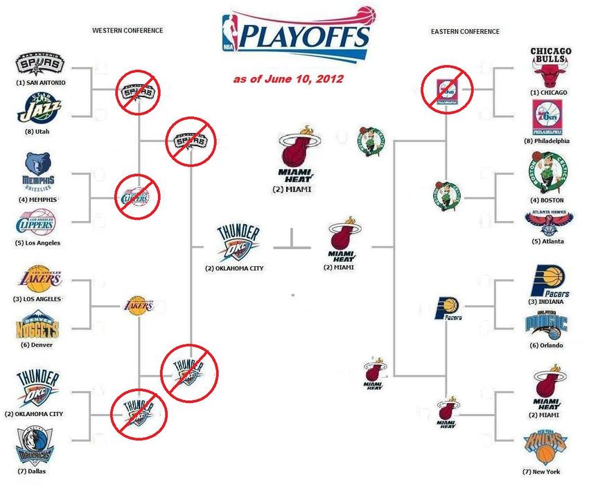
APPENDIX I NBA 2012

After finding the best models, these are used to predict the playoffs of 2012. Using the K-nn
model, with the best binomial based performance, the playoffs are predicted as figure 6 shows.

FIGURE 6: PERFORMANCE OF THE FINAL K-NN 15 MODEL ON THE 2012 PLAYOFFS. THE RED
ENCIRCLED TEAMS ARE PREDICTED WRONG BY THE MODEL.

As this figure shows, the model did not perform well on this particular year. One interesting fact
is the predicting on both nr1-nr8 games. While the mispredicting on the Bulls is imaginable, the
model predicts the Utah Jazz defeat the Spurs. Both where the model predicts the number 8 to
defeat the number 1 and the number 1 to defeat the number 8, the opposite happens.
Most of the false predictions are to be found in the left side of the figure, the western conference.
The false prediction of the Grizzlies-Clippers game is imaginable because the Memphis Grizzlies
had performed better during the season and they thereby had the home-advantage. In most
cases this team wins, so the Clippers win can be called unusual. Problems predicting the
Thunder-Mavericks and the Lakers-Thunder games are more unusual. The model predicts the
Thunder to lose both times, while the Thunder had the home-advantage and the better
performance during the regular season. The models decision might thereby be based on the
shooting percentages. In total the model performs 60% on this season’s playoffs, but it does
predict the winner right.

25
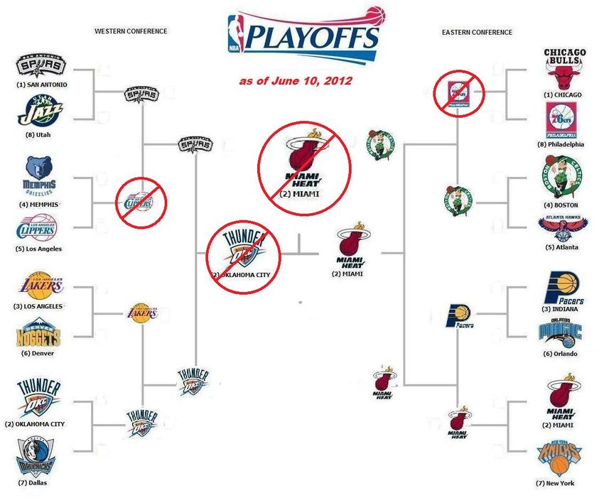
FIGURE 7: PERFORMANCE OF THE FINAL NAÏVE BAYES MODEL ON THE 2012 PLAYOFFS. THE
RED ENCIRCLED TEAMS ARE PREDICTED WRONG BY THE MODEL.

Figure 7 shows the results of the, probability based, best performing model, on the 2012
playoffs. Again, just as the K-nn model from figure 6, this model has problems with the Bulls-
76’ers and the Grizzlies-Clippers games. Again, this is imaginable because the losing team had a
better     winning     percentage     during     the   season     and   the     home-advantage.
It is interesting to see the model, for this season, only predicting wins for the team with the
home-advantage. In this case this results in a performance of 74,11%.

26
You can also read