QMCPACK: Advances in the development, efficiency, and application of auxiliary field and real-space variational and diffusion Quantum Monte Carlo
←
→
Page content transcription
If your browser does not render page correctly, please read the page content below
QMCPACK: Advances in the development, efficiency, and application of auxiliary
                                                  field and real-space variational and diffusion Quantum Monte Carlo

                                                             P. R. C. Kent,1, a) Abdulgani Annaberdiyev,2 Anouar Benali,3 M. Chandler Bennett,4
                                                             Edgar Josué Landinez Borda,5 Peter Doak,6 Hongxia Hao,7 Kenneth D. Jordan,8
                                                             Jaron T. Krogel,9 Ilkka Kylänpää,10 Joonho Lee,11 Ye Luo,3 Fionn D. Malone,5 Cody
arXiv:2003.01831v2 [physics.comp-ph] 6 May 2020

                                                             A. Melton,12 Lubos Mitas,2 Miguel A. Morales,5 Eric Neuscamman,7, 13 Fernando A.
                                                             Reboredo,9 Brenda Rubenstein,14 Kayahan Saritas,15 Shiv Upadhyay,8 Guangming
                                                             Wang,2 Shuai Zhang,16 and Luning Zhao17
                                                             1)
                                                                  Center for Nanophase Materials Sciences Division and Computational
                                                             Sciences and Engineering Division, Oak Ridge National Laboratory, Oak Ridge,
                                                             Tennessee 37831, USAb)
                                                             2)
                                                                  Department of Physics, North Carolina State University, Raleigh,
                                                             North Carolina 27695-8202, USA
                                                             3)
                                                                  Computational Science Division, Argonne National Laboratory,
                                                             9700 S. Cass Avenue, Lemont, IL 60439, USA
                                                             4)
                                                                  Materials Science and Technology Division, Oak Ridge National Laboratory,
                                                             Oak Ridge, Tennessee, 37831, USA
                                                             5)
                                                                  Quantum Simulations Group, Lawrence Livermore National Laboratory,
                                                             7000 East Avenue, Livermore, CA 94551, USA
                                                             6)
                                                                  Center for Nanophase Materials Sciences Division and Computational
                                                             Sciences and Engineering Division, Oak Ridge National Laboratory, Oak Ridge,
                                                             Tennessee 37831, USA
                                                             7)
                                                                  Department of Chemistry, University of California, Berkeley, California 94720,
                                                             USA
                                                             8)
                                                                  Department of Chemistry, University of Pittsburgh, Pennsylvania 15260,
                                                             USA
                                                             9)
                                                                  Materials Science and Technology Division, Oak Ridge National Laboratory,
                                                  b)
                                                       Notice:     This manuscript has been authored by UT-Battelle, LLC, under Contract No.                DE-

                                                       AC0500OR22725 with the U.S. Department of Energy. The United States Government retains and the

                                                       publisher, by accepting the article for publication, acknowledges that the United States Government re-

                                                       tains a non-exclusive, paid-up, irrevocable, world-wide license to publish or reproduce the published form

                                                       of this manuscript, or allow others to do so, for the United States Government purposes. The Department

                                                       of Energy will provide public access to these results of federally sponsored research in accordance with
                                                                                                        1
                                                       the DOE Public Access Plan (http://energy.gov/downloads/doe-public-access-plan)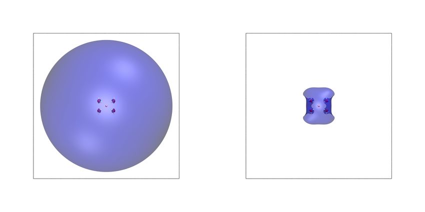
Oak Ridge, Tennessee 37831, USA
10)
      Computational Physics Laboratory, Tampere University, P.O. Box 692,
33014 Tampere, Finland
11)
      Department of Chemistry, Columbia University, New York, NY 10027,
USA
12)
      Sandia National Laboratories, Albuquerque, New Mexico 87123,
USA
13)
      Chemical Sciences Division, Lawrence Berkeley National Laboratory, Berkeley,
CA, 94720, USA
14)
      Department of Chemistry, Brown University, Providence, RI 02912,
USA
15)
      Department of Applied Physics, Yale University, New Haven, CT 06520,
USA
16)
      Laboratory for Laser Energetics, University of Rochester, 250 E River Rd,
Rochester, NY 14623, USA
17)
      Department of Chemistry, University of Washington, Seattle, Washington, 98195,
USA

(Dated: 7 May 2020)

                                       2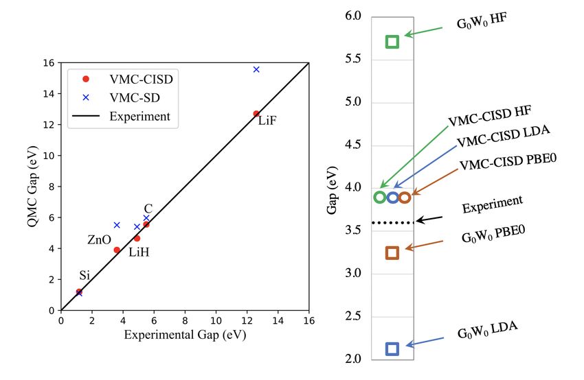
We review recent advances in the capabilities of the open source ab initio Quan-
           tum Monte Carlo (QMC) package QMCPACK and the workflow tool Nexus used
           for greater efficiency and reproducibility. The auxiliary field QMC (AFQMC) im-
           plementation has been greatly expanded to include k-point symmetries, tensor-
           hypercontraction, and accelerated graphical processing unit (GPU) support. These
           scaling and memory reductions greatly increase the number of orbitals that can prac-
           tically be included in AFQMC calculations, increasing accuracy. Advances in real
           space methods include techniques for accurate computation of band gaps and for
           systematically improving the nodal surface of ground state wavefunctions. Results
           of these calculations can be used to validate application of more approximate elec-
           tronic structure methods including GW and density functional based techniques.
           To provide an improved foundation for these calculations we utilize a new set of
           correlation-consistent effective core potentials (pseudopotentials) that are more ac-
           curate than previous sets; these can also be applied in quantum-chemical and other
           many-body applications, not only QMC. These advances increase the efficiency, ac-
           curacy, and range of properties that can be studied in both molecules and materials
           with QMC and QMCPACK.

a)
     kentpr@ornl.gov

                                                3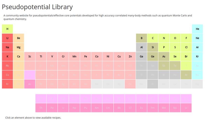
I.    INTRODUCTION

     Quantum Monte Carlo (QMC) methods are an attractive approach for accurately com-
puting and analyzing solutions of the Schrödinger equation.1–3 The methods form a general
ab initio methodology able to solve the quantum many-body problem, applicable to idealized
models such as chains or lattices of atoms through to complex and low-symmetry molec-
ular and condensed matter systems, whether finite or periodic, metallic or insulating, and
with weak to strong electronic correlations. Significantly, the methods can naturally treat
systems with significant multi-reference character, and are without electron self-interaction
error, which challenges many quantum chemical approaches and density functional theory
approximations, respectively. The methods continue to be able to take advantage of im-
provements in computational power, giving reduced time to solution with new generations
of computing. Due to these features, usage of QMC methods for first principles and ab initio
calculations is growing.

     Compared to traditional deterministic approaches, QMC methods are generally distin-
guished by: (1) use of statistical methodologies to solve the Schrödinger equation. This
allows the methods to not only treat problems of high-dimensionality efficiently, but also
potentially use basis, wave function, and integral forms that are not amenable to numerical
integration. (2) Use of few and well-identified approximations that can potentially be quan-
tified or made systematically convergeable. (3) A low power scaling with system-size, but
large computational cost prefactor. (4) High suitability to large scale parallel computing ow-
ing to lower communications requirements than conventional electronic structure methods.
Scaling has been demonstrated to millions of compute cores.4

     Modern applications of QMC have expanded to cover many of the same systems studied
by density functional theory (DFT) and quantum chemical approaches, and in many cases
also at a similar atom and electron count, although at far greater computational cost. Besides
those described in below, recent molecular applications of QMC include studies of the nature
of the quadruple bond in C2 5 , acenes6 , physisorption of water on graphene7 , binding of
transition metal diatomics8 , and DNA stacking energies9 . Materials applications include
nitrogen defects in ZnO10 , excitations in Mn doped phosphors11 , and the singlet-triplet
excitation in MgTi2 O4 12 . Methodological improvements include: reducing the sensitivity
of pseudopotential evaluation13 , extensions to include linear response14 , density functional

                                             4
embedding15 , excited states including geometry optimization16 , improved twist averaging17 ,
and accurate trial wavefunctions via accurate densities18 . Importantly, for model systems
such as the hydrogen chain, the methods can be used to benchmark themselves as well as
other many-body approaches19 . This partial list of developments and applications from the
last two years alone indicates that the field is growing and maturing.
In this article we describe recent updates to the QMCPACK code and its ecosystem
of wavefunction converters and workflow tools. These updates have aimed to expand the
range of systems, properties, and accuracies that can be achieved both with QMCPACK
and with QMC techniques in general. For a description of the underlying methodology we
refer the reader to Refs. 1–4, and 20. In particular, a thorough description of real space
QMC methods is given in Section 5 of Ref. 4. For an extensive introduction to AFQMC we
refer the reader to Ref.20.
QMCPACK is a fully open source and openly developed QMC package, with 48 coauthors
on the primary citation paper4 published in 2018 and an additional 5 contributors since then.
The main website for QMCPACK is https://qmcpack.org and the source code is currently
available through https://github.com/QMCPACK/qmcpack. QMCPACK aims to implement
state of the art QMC methods, be generally applicable, easy to use, and high-performing on
all modern computers. Since the publication of Ref.4 , the range of QMC calculations that
are possible has been expanded by significant enhancements to the Auxiliary-Field QMC
(AFQMC) solver. This orbitally based method is distinct from and complementary to the
longer-implemented real space methods of variational and diffusion QMC (VMC and DMC,
respectively). The AFQMC implementation can fully take advantage of graphics processing
units (GPUs) for a considerable speedup and, unlike the real-space methods, can also exploit
k-point symmetries. It shares the same workflow tool, Nexus, which helps simplify and ease
application of all the QMC methods by new users as well as aid in improving reproducibility
of complex multi-step research investigations. To our knowledge this is currently the only
AFQMC code designed for large scale research calculations that is open source. To help
guarantee the future of the code, it is undergoing rapid development and refactoring to target
the upcoming Exascale architectures as part of the U.S. Exascale Computing Project21 ,
which also entails major updates to the testing, validation and maintainability.
The electronic structure and quantum chemical codes that QMCPACK is interfaced to for
trial wavefunctions has been expanded to include Qbox22 , PySCF23 , Quantum Espresso24 ,
5Quantum Package25 , and GAMESS26 . Additional codes such as NWCHEM27 can be inter-
faced straightforwardly.
In the following, we first review in Section II the open development principles of QMC-
PACK. In Section III we discuss updates to the Nexus workflow package. This integrates
entire research electronic structure workflows for greater productivity and reproducibility
than by-hand invocation of individual calculations. Due to the infeasibility of performing
QMC calculations for general systems using an all electron approach, use of effective core
potentials (ECPs), or pseudopotentials, is essential. To improve the accuracy obtainable
we have developed a new approach and set of “correlation consistent” ECPs. These can
be used in all ab initio calculations, not only QMC, and are described in Section IV. Ad-
vances in the AFQMC implementation are described in Section V. Turning to real-space
QMC methods in Section VI, algorithms and multiple determinant trial wavefunctions can
now be used to obtain improved ground state energies as well as band gaps in solid-state
materials. As a result, it is now possible to begin to test the accuracy of the nodal surfaces
that have long been used in these calculations. Finally, in Section VII, we give three ap-
plications: first, application to non-valence anions, which challenge all electronic structure
and quantum chemical techniques. Second, application to excitations of localized defects
in solids VII B. Third, the ability to obtain the momentum distribution has recently been
improved, motivated by recent experiments on VO2 . A summary is given in Section VIII.
II. OPEN DEVELOPMENT AND TESTING
Fully open source development is an important core value of the QMCPACK develop-
ment team. Besides improving the quality of the software, anecdotally it also improves the
on-boarding experience for new users. While the developers of many electronic structure
packages now practice some degree of open development, QMCPACK has seen very signif-
icant benefits from this in the last few years. We expect other packages would also benefit
from full adoption and therefore give details here.
QMCPACK is an open source package, with releases and the latest development source
code available through https://github.com/QMCPACK/qmcpack. QMCPACK is written in
C++14, with MPI parallelization between compute nodes, OpenMP threading used for
multicore parallelism. CUDA is used for NVIDIA accelerators. Options to support CUDA,
6complex valued wavefunctions, and to adjust the numerical precision used internally are
currently compile time options.
Besides adoption of a distributed source code control system, we have found that devel-
opment productivity can be further increased by adoption of code reviews and continuous
integration (testing). To maximize the efficiency of both contributors and reviewers and
shorten the development cycle of new features, work-in-progress pull requests are encour-
aged for early engagement in the process. The early review allows guidance to be given,
e.g. are the algorithms clear enough to other developers and are the coding guidelines being
followed. At the same time, continuous integration is applied to the proposed code change.
This process routinely catches cases that developers may not have considered or tested
against, e.g. the complex-valued build of QMCPACK or accelerated GPU support, that are
compile time options. This period of comment while the work is being completed also helps
advertise the work to other developers and minimizes risk of duplicated work. Our experi-
ence strongly suggests that this process reduces bugs, reduces potential developer’s effort,
and saves reviewer’s time compared to a late engagement with an unexpected pull request.
All the discussions around the code change become archived searchable documentation and
potential learning materials.
Testing of QMCPACK has been significantly expanded. Two years ago, QMCPACK had
limited unit, integration and performance testing categories: unit tests that run quickly on
individual components; integration tests that exercise entire runs; performance tests for mon-
itoring relative performance between code changes. However, due to the stochastic nature
of QMC, as the number of tests and build combinations increased it became impractical to
run the integration tests long enough to obtain a statistically reliable pass/fail: the smallest
(shortest) integration test set currently takes around one hour to execute on a 16 core ma-
chine, and must necessarily suffer from occasional statistical failures. Thus, a new category
of tests was needed for quickly examining full QMC execution with a reproducible Monte
Carlo trajectory. The new deterministic integration tests are modified QMC runs with only
a few steps, very few Monte Carlo walkers, and fixed random seeds for absolute reproducibil-
ity. All the major features of QMCPACK are covered by this new of category tests. Running
all the unit and deterministic integration tests takes approximately one minute which is fast
enough for iterative development and fast enough to be used in continuous integration. This
fast to run set of tests facilitates significant changes and refactoring of the application which
7otherwise would be far more difficult to test and unlikely to be attempted by non-experts
without long experience with the codebase. All the deterministic tests are accompanied
by longer running statistical tests that can be used to verify a new implementation when
changes alter a previous deterministic result. Combinations of these tests are run automat-
ically on a nightly basis and report to a public dashboard https://cdash.qmcpack.org.
At the time of writing, around 25 different machine and build combinations are used to run
around 1000 labeled tests each, and most of these cover multiple features.
Improving source code readability is critical for both new and experienced developers. In
the past, misleading variable or class names and confusing function names have confused
developers and resulted in subtle bugs, e.g. due to similarly named functions, only one of
which updates internal state in the Monte Carlo algorithm. For this reason, coding standards
including naming conventions have been added in the manual and are enforced on newly
contributed codes. Existing codes are updated to follow the standards as they need other
modifications. Automatic source formatting is also applied with the help of the clang-format
tool. Concomitantly, both developer sections in the manual and source code documentation
are significantly expanded.
As a result of the above changes, new contributors with a basic theoretical background
can connect source code with textbook equations with much less difficulty than in the past.
These efforts are clearly bringing long term benefit to QMCPACK and hopefully can be
transferred to other scientific applications as well.
III. IMPROVING QMC WORKFLOWS WITH NEXUS
QMC techniques are progressing from methods under research towards more routine
application. In this transition, usability of QMC becomes an important factor. A mature,
usable computational method transfers responsibility for correct execution from users to
the code. Major factors determining overall usability include: ease of requesting a desired
result (in the form of input), robustness of the code in obtaining the desired result, and
complexity of the overall calculation process. All of these contribute to the effort required
by the user to obtain desired results. In essence, higher required effort translates directly
into lower productivity of the user base. Lower productivity in turn risks a lower overall
adoption rate and thus blunts overall impact of the method. It is therefore important to
8seek to understand and minimize barriers to the practical use of QMC.
To illustrate the complexity of the QMC calculation process, we describe below a basic
but realistic sequence of calculations (a scientific workflow) that is required to obtain a final
fixed node DMC total energy per formula unit for a single crystalline solid with QMCPACK.
In this workflow, we suppose that self-consistent (SCF) and non-self-consistent (NSCF)
calculations are performed with Quantum Espresso24 and wavefunction optimization (OPT),
variational Monte Carlo (VMC), and diffusion Monte Carlo calculations are performed with
QMCPACK. SCF/NSCF calculations might be performed on a workstation or a few nodes
of a cluster, VMC/OPT calculations on a research-group sized cluster (∼30 nodes), and
DMC on high performance computing resources (∼1000 nodes).
1. Converge DFT orbitals with respect to plane-wave energy cutoff (4–6 SCF calculations
ranging from 300 to 800 Ry for the energy cutoff).
2. Converge B-spline orbital representation with respect to B-spline mesh spacing (1
NSCF, ∼5 VMC calculations in a small supercell over a series of finer mesh spacings).
3. Converge twist grid density (∼5 VMC calculations in a small supercell for a series of
increasingly dense supercell Monkhorst-Pack twist grids).
4. Determine best optimization process (∼6 optimization (OPT) calculations in a small
supercell over varying input parameters and e.g. Jastrow forms).
5. Obtain fixed node DMC total energy (∼3 NSCF, ∼3 OPT and ∼9 DMC calcula-
tions, 3 successively smaller timesteps for timestep extrapolation, 3 successively larger
supercells for finite size extrapolation).
This basic workflow process is to be compared with the much reduced complexity for
obtaining a single converged total energy for DFT, which typically requires only a single
input file and single program execution to perform a single SCF calculation for the final
energy. The complexity intrinsic to the basic workflow translates into a large degree of
effort on the part of the user and limits the accessibility of the method for new users or
for experienced users pursuing ambitious projects comprised of a large number of DMC
calculations.
9Scientific workflow tools make the QMC process more accessible in multiple ways: (1)
bringing the constellation of electronic structure codes needed to produce a single QMC
result under a single framework, (2) reducing the number of inputs required to request a
desired result to a single user-facing input file, (3) reducing overall complexity by abstracting
the execution process, (4) minimizing the direct effort required to execute the workflow
process by assuming the management of simulation execution and monitoring from the user.
Workflow tools have been applied with significant benefit to related electronic structure
methods such as DFT28–31 and also to QMC32,33 .
The Nexus workflow automation system34 was created to realize these advantages for users
of QMCPACK. Nexus is a Python-based, object oriented workflow system that can be run on
a range of target architectures. Nexus has been used successfully on simple workstations and
laptops, small group or institutional computing clusters, university level high performance
computing centers in the U.S. and internationally, and Leadership Computing Facilities
supported by the U.S. Department of Energy. Nexus has been used in a growing number of
QMC studies involving QMCPACK and its uptake by new users is high.
Nexus abstracts user’s interactions with each target simulation code that are components
of a desired simulation workflow. Access to each respective code is enabled through single
function calls that only require the user to specify a reduced set of important input param-
eters. Each function call resembles a small input block from a standard input file for an
electronic structure code. Taken together, a sequence of these blocks comprises a new meta-
input file that represents the data flow and execution pattern of the underlying simulation
codes as a combined workflow.
Nexus assumes the responsibility of initiating and monitoring the progress of each sim-
ulation job in the workflow. Nexus generates expanded input files to each code based on
the reduced inputs provided by the user. It also generates job submission files and monitors
job execution progress via a lightweight polling mechanism. Apart from direct execution of
each workflow step, Nexus also automates some tasks that previously fell to users. One ex-
ample is that Nexus selects the best wavefunction produced during the non-linear statistical
optimization process employed by QMCPACK and automatically passes this wavefunction
to other calculations (such as diffusion Monte Carlo), which require it.
In the future, additional productivity gains might be realized with Nexus by further ab-
stracting common workflow patterns. For example, convergence studies for orbital param-
10eters (k-points, mesh-factors, source DFT functional) often follow similar patterns which
could be encapsulated as simple components for users. Additionally, more of the responsi-
bility for obtaining desired results, e.g. total energies to a statistically requested tolerance,
could be handled by Nexus through algorithms that create and monitor dynamic workflows.
IV. EFFECTIVE CORE POTENTIALS
A. Introduction
All-electron (AE) QMC calculations become inefficient and eventually infeasible with in-
creasing atomic number Z since the computational cost grows roughly as35,36 Z 6 . Since our
primary interest is in valence properties, pseudopotentials and/or effective core potentials
(ECP) are commonly employed to eliminate the atomic cores leading to valence-only effec-
tive Hamiltonians. Unfortunately, the existing tables and ECP generating tools have proved
to exhibit somewhat mixed fidelity to the true all-electron calculations, especially in high
accuracy QMC studies. In order to overcome this limitation, we have proposed and con-
structed a new generation of valence-only Hamiltonians called correlation consistent ECPs
(ccECP)37–40 . The key feature of this new set is the many-body construction of ccECPs
from the outset, in particular: (i) we have emphasized and put upfront the accuracy of
many-body valence spectra (eigenvalues and eigenstates) as a guiding principle in addition
to the well-known norm conservation/shape consistency principles; (ii) we have opted for
simplicity, transparency and eventual wide use, in addition to offering several choices of
core sizes or even smoothed-out all-electron nuclear Coulomb potentials; (iii) we have used
a set of tests and benchmarks such as molecular bonds over a range of distances in order to
extensively probe for the quality and transferability of the ccECPs; (iv) we have established
reference data sets for the exact/nearly-exact atomic total energies, kinetic energies, as well
as single-reference and multi-reference fixed-node DMC energies. At present, this covers
elements H-Kr with subsequent plans to fill the periodic table.
B. ccECP atomic and molecular properties.
The construction of ccECPs builds in electron correlations obtained from the accurate
coupled-cluster singles doubles with perturbative triples (CCSD(T)) method. By doing so,
11ccECPs achieve very high accuracy and enjoy spectral properties on the valence subspace
that are in close agreement with the scalar relativistic all-electron (AE) Hamiltonian. The
agreement is often within chemical accuracy over a large range of atomic excitations and
ionizations that often spans hundreds of eV energy windows. Molecular properties such
as binding energies in multiple geometries, equilibrium bond lengths, and vibrational fre-
quencies were also considered in the development, mostly examining oxides, hydrides, and
homonuclear dimers. Especially, compressed bond length properties were given priority as
this corresponds to high-pressure applications and probes for the proper behavior of the
valence charge in the core region. These atomic and molecular tests provide a direct and
comprehensive comparison of ccECP and other core approximations such as BFD41 , STU42 ,
eCEPP43 , CRENBL44 , SBKJC45 , UC (uncorrelated, self-consistent, all-electron core), and
ccECP.S (optimization including only atomic spectrum). Here we illustrate some of these
results for selected cases.
Figure 1 shows the molecular binding energy discrepancies for FeH, FeO, VH, and VO
molecules relative to all-electron CCSD(T) where we observe that some previous ECPs
display significant errors. In addition, Table I, lists a more comprehensive comparison by
tabulating the average of mean absolute deviations (MAD) of molecular binding properties
relative to all-electron CCSD(T) for all 3d transition metal (TM) molecules. Similarly,
Figure 2a presents the MAD of a large valence spectrum for all 3d TM atoms. In both atomic
and molecular tests, we see that ccECP achieves smaller or on par average errors with regard
to the other ECPs. In addition, Fig. 1 shows these improvements to be consistent for different
elements and varying geometries. Hence, we believe that ccECP accomplishes the best
accuracy compromise for atomic spectral and molecular properties. Furthermore, ccECPs
are provided with smaller cores than conventionally used ones in some cases where large
errors were observed. This includes Na-Ar with [He] core and H-Be with softened/canceled
Coulomb singularity at the origin (ccECP(reg)). Selected molecular test results for these
are shown in Figure 3.
For reference, we also provide accurate total and kinetic energies for all ccECPs46 using
methods such as CCSDT(Q)/FCI (FCI, full configuration interaction) with DZ-6Z extrap-
olations to estimate the complete basis set limit. This data, for instance, is useful in the
assessment of fixed-node DMC biases. Figure 2b shows the summary of single-reference
(HF) fixed-node DMC errors for ccECP pseudo atoms.
12UC eCEPP
BFD ccECP.S
0.10 STU ccECP 0.05
Discrepancy (eV)
Discrepancy (eV)
0.00
0.05
−0.05
0.00 −0.10
UC eCEPP
BFD ccECP.S
−0.15 STU ccECP
−0.05
1.2 1.4 1.6 1.8 1.2 1.4 1.6 1.8
Bond Length (Å) Bond Length (Å)
(a) FeH binding curve discrepancies. (b) FeO binding curve discrepancies
0.100 UC UC
BFD BFD
STU 0.3 STU
0.075
Discrepancy (eV)
eCEPP Discrepancy (eV) eCEPP
ccECP.S ccECP.S
0.050 ccECP 0.2 ccECP
0.025
0.1
0.000
−0.025 0.0
−0.050
1.2 1.4 1.6 1.8 2.0 1.2 1.3 1.4 1.5 1.6 1.7
Bond Length (Å) Bond Length (Å)
(c) VH binding curve discrepancies (d) VO binding curve discrepancies
FIG. 1: Binding energy discrepancies for (a) FeH, (b) FeO, (c) VH, and (d) VO molecules.
The binding curves are relative to scalar relativistic AE CCSD(T) binding curve. The
shaded region indicates a discrepancy of chemical accuracy in either direction. The
ccECPs are the only valence Hamiltonians that are consistently within the shaded region
of chemical accuracy including short bond lengths which are relevant for high pressures.
Reproduced from Ref. 39, with the permission of AIP Publishing.
C. ccECP Database and Website
In order to facilitate the use ccECPs, we have provided basis sets and a variety of ECP
formats available at https://pseudopotentiallibrary.org, shown in Figure 4. Each
ccECP is presented in a quantum chemistry format for direct use in various codes, including
13UC BFD STU eCEPP ccECP.S ccECP
De (eV) 0.0063(40) 0.0590(41) 0.0380(41) 0.0163(45) 0.0240(40) 0.0104(40)
re (Å) 0.0012(13) 0.0064(13) 0.0026(13) 0.0019(15) 0.0027(13) 0.0010(13)
ωe (cm−1 ) 2.2(5.8) 10.4(5.9) 4.6(5.9) 3.9(6.9) 6.4(5.8) 2.9(5.8)
Ddiss (eV) 0.021(41) 0.145(41) 0.036(41) 0.032(46) 0.054(40) 0.016(41)
TABLE I: Average MADs of binding parameters for various core approximations with
respect to AE data for 3d TM hydride and oxide molecules. All parameters were obtained
using Morse potential fit. The parameters shown are dissociation energy De , equilibrium
bond length re , vibrational frequency ωe and binding energy discrepancy at dissociation
bond length Ddiss . Reproduced from Ref. 39, with the permission of AIP Publishing.
UC eCEPP 12
2.0
Mean Absolute Deviation (eV)
BFD ccECP.S
STU ccECP 10
1.5 8
Percentage
6
1.0
Be-Ne[He]
4
Mg-Ar[Ne]
0.5 2 Na-Ar[He]
Ga-Kr[[Ar]3d10 ]
0 K-Zn[Ne]
0.0
1 2 3 4 5 6 7 8 9 10 11 12
Sc Ti V Cr Mn Fe Co Ni Cu Zn Number of valence electrons
(a) (b)
FIG. 2: (a) MADs for 3d TM benchmark states from bare [Ne] core up to low-lying neutral
excitations and the anionic state. (b) Fixed-node DMC biases () as a percentage of the
correlation energy for ccECP pseudo atoms: 100/|Ecorr |. T-moves47 and single-reference
trial functions were used in calculations with the exception of Be, B, and C with
two-reference form to account for the significant 2s − 2p near-degeneracy. Fig. 2a
reproduced from Ref. 39, with the permission of AIP Publishing. Fig. 2b is adapted with
permission from Ref. 46. Copyright 2020 American Chemical Society.
140.2 0.2
0.0
Discrepancy (eV)
Discrepancy (eV)
0.0
−0.2
−0.2
UC
BFD
−0.4 UC
−0.4 SDFSTU SBKJC
eCEPP −0.6 BFD
SBKJC TN-DF
−0.6 CRENBL STU
ccECP −0.8 ccECP[Ne]
ccECP(reg) ccECP[He]
−0.8 −1.0
1.2 1.4 1.6 1.8 1.2 1.3 1.4 1.5 1.6
Bond Length (Å) Bond Length (Å)
(a) LiO binding curve discrepancies (b) SiO binding curve discrepancies
FIG. 3: Binding energy discrepancies for (a) LiO and (b) SiO molecules. The uncorrelated
core (UC) results, plus those for many different effective core potentials are given relative
to scalar relativistic all electron (AE) CCSD(T) binding curve. The shaded region indicates
a discrepancy of chemical accuracy in either direction. Details are given in Refs. 38 and 40.
Reproduced from Ref. 40 and Ref. 38, with the permission of AIP Publishing.
Molpro, GAMESS, NWChem, and PySCF which uses the NWChem format. We also
provide an XML format which can directly be used in QMCPACK.
In addition to the ccECPs themselves, we have also provided basis sets appropriate for
correlated calculations in each code format. Specifically, we have provided Dunning style48
correlation consistent basis sets from the DZ to 6Z, and in most cases have also provided
an augmented version. For use in solid state applications using a plane wave basis, we have
also transformed the semi-local potentials into fully nonlocal Kleinman-Bylander potentials49
using the Unified Pseudopotential Format. This allows the ccECPs to be directly used in
codes such as Quantum Espresso. A report file is included giving detailed information
about the quality of the Kleinman-Bylander version of the potential and recommended plane
wave energy cutoff energies.
D. Status and future developments
The ccECP table and construction principles aim at improved account of systematic errors
built into effective valence Hamiltonians in a wide variety of correlated calculations (see
15FIG. 4: Pseudopotential Library, https://pseudopotentiallibrary.org.
encouraging feedback so far50,51 ). Further effort is focused on adapting ccECPs for efficient
calculations with plane wave basis set (ccECPpw versions). This requires modifying the deep
potentials of the late 3d elements Fe-Zn in particular. The goal is to enable calculations with
plane wave cutoffs not exceeding ∼ 600-800 Ry. Plans for the near future involve ccECPs
for selected 4d and 5d elements that include a number of technologically important elements
and require explicit treatment of the spin-orbit interactions. Additional improvements such
as core polarization and relaxation corrections can be added per specific, application driven
needs. Further plans include seeking feedback from the electronic structure community,
collecting the data for reference and validation as well as adjustments per need for use in a
broad variety of ab initio approaches.
V. AUXILIARY FIELD QUANTUM MONTE CARLO
The latest version of QMCPACK offers a now mature implementation of the phase-
less auxiliary-field quantum Monte Carlo (AFQMC) method20,52 capable of simulating both
molecular53,54 and solid state systems55–57 . AFQMC is usually formulated as an orbital-space
approach in which the Hamiltonian is represented in second-quantized form as
X 1X
Ĥ = hij ĉ†i ĉj + vijkl ĉ†i ĉ†j ĉl ĉk + EII , (1)
ij
2 ijkl
= Ĥ1 + Ĥ2 + EII , (2)
16where ĉ†i and ĉi are the fermionic creation and annihilation operators, hij and vijkl are the one-
and two-electron matrix elements and EII is the ion-ion repulsion energy. Key to an efficient
implementation of AFQMC is the factorization of the 4-index electron-repulsion integral
(ERI) tensor vijkl , which is essential for the Hubbard-Stratonovich (HS) transformation58,59 .
QMCPACK offers three factorization approaches which are appropriate in different
settings. The most generic approach implemented is based on the modified-Cholesky
factorization60–64 of the ERI tensor:
N
X chol
vijkl = V(ik),(lj) ≈ Lnik L∗n
lj , (3)
n
where the sum is truncated at Nchol = xc M , xc is typically between 5 and 10, M is the
number of basis functions and we have assumed that the single-particle orbitals are in general
complex. The storage requirement is thus naively O(M 3 ) although sparsity can often be
exploited to keep the storage overhead manageable (see Table II). Note that QMCPACK
can accept any 3-index tensor of the form of Lnik so that alternative density-fitting based
approaches can be used. Although the above approach is efficient for moderately sized
molecular and solid-state systems, it is typically best suited to simulating systems with
fewer than 2000 basis functions.
To reduce the memory overhead of storing the three-index tensor we recently adapted
the tensor-hypercontraction65–67 (THC) approach for use in AFQMC56 . Within the THC
approach we can approximate the orbital products entering the ERIs as
Nµ
X
ϕ∗i (r)ϕk (r) ≈ ζµ (r)ϕ∗i (rµ )ϕk (rµ ), (4)
µ
where ϕi (r) are the one-electron orbitals and rµ are a set of specially selected interpolating
points, ζµ (r) are a set of interpolating vectors and Nµ = xµ M . We can then write the ERI
tensor as a product of rank-2 tensors
X
vijkl ≈ ϕ∗i (rµ )ϕk (rµ )Mµν ϕ∗j (rν )ϕl (rν ), (5)
µν
where
1
Z
Mµν = drdr0 ζµ (r) ζ ∗ (r0 ). (6)
|r − r0 | ν
To determine the interpolating points and vectors we use the interpolative separable density
fitting (ISDF) approach68–70 . Note that the storage requirement has been reduced to O(M 2 ).
17For smaller system sizes the three-index approach is preferred due to the typically larger
THC prefactors determined by xµ ≈ 15 for propagation and xµ ≈ 10 for the local energy
evaluation. The THC approach is best suited to simulating large supercells, and is also
easily ported to GPU architectures due to its smaller memory footprint and use of dense
linear algebra. Although the THC-AFQMC approach has so far only been used to simulate
periodic systems, it is also readily capable of simulating large molecular systems using the
advances from Ref. 71.
Finally, we have implemented an explicitly k-point dependent factorization for periodic
systems72
nQ
chol
X Qkl ∗
V(ikk +Qkkk ),(lkl jkl −Q) ≈ LQk
ik,n Llj,n ,
k
(7)
n
where now i runs over the number of basis functions (m) for k-point ki in the primitive cell,
Q = ki − kk + G = kl − kj + G0 is the momentum transfer vector (arising from the conser-
vation of crystal momentum) and G, G0 are reciprocal lattice vectors. Although explicitly
incorporating k-point symmetry reduces the scaling of many operations and the storage
requirement by a factor of 1/Nk (see Table. II), perhaps the most significant advantage is
that it permits the use of batched dense linear algebra and is thus highly efficient on GPU
architectures. Note that the THC and k-point symmetric factorization can be combined to
simulate larger unit cells and exploit k-point symmetry, however this has not been used to
date. We compare the three approaches in Table II and provide guidance for their best use.
In addition to state-of-the-art integral factorization techniques, QMCPACK also permits
the use of multi-determinant trial wavefunction expansions of the form
ND
X
|ψT i = cI |DI i. (8)
I
We allow for either orthogonal configuration interaction expansions where hDI |DJ i = δIJ and
also for non-orthogonal multi Slater determinant expansions (NOMSD) where hDI |DJ i =
SIJ . Orthogonal expansions from complete active space self-consistent field (CASSCF) or
selected CI methods allow for fast overlap and energy evaluation through Sherman-Morrison
based techniques, and thus do not typically incur a significant slowdown. However, they often
require a large number of determinants to converge the phaseless error. NOMSD expansions
do not benefit from fast update techniques, but often require orders of magnitude fewer
18Method Memory Propagation Energy Setting GPU
Dense 3-index xc M 3 O(N M 2 ) O(xc N 2 M 2 ) M ≤ 1000 Yes
Sparse 3-index sxc M 3 O(N M 2 ) O(N 2 M 2 ) M ≤ 2000 No
THC x2µ M 2 O(N M 2 ) O(x2µ N M 2 ) M ≤ 4000 No
k-point xc m3 Nk2 O(N M 2 ) O(xc m2 n2 Nk3 ) Nk m ≤ 6000 Yes
TABLE II: Comparison in the dominant scaling behavior of different factorization
approaches implemented in QMCPACK. We have included a sparsity factor s which can
reduce the computational cost of the three-index approach significantly. For example, in
molecular systems the memory requirement is asymptotically O(M 2 ) in the atomic orbital
basis, whilst for systems with translational symmetry the scaling is in principle identical to
that of the explicitly k-point dependent factorization (i.e. s ≤ 1/Nk ) although currently
less computationally efficient. We also indicate the current state of GPU support for the
different factorizations available in QMCPACK. The THC factorization will be ported to
GPUs in the near future. Note that by using plane waves the scaling of the energy
evaluation and propagation can be brought down to O(N 2 M log M ) and O(N M log M )
respectively. This approach essentially removes the memory overhead associated with
storing the ERIs at the cost of using a potentially very large plane-wave basis set73,74 . This
plane wave approach is not yet available in QMCPACK.
determinants than their orthogonal counterparts to achieve convergence in the AFQMC
total energy53 (see Fig. 5).
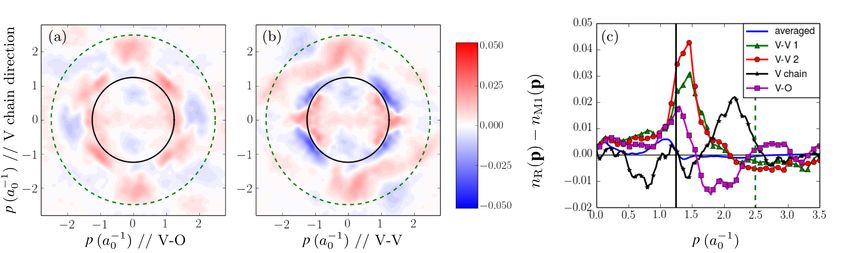
QMCPACK also permits the evaluation of expectation values of operators which do not
commute with the Hamiltonian using the back propagation method59,81,82 . In particular,
the back-propagated one-particle reduced density matrix (1RDM) as well components or
contracted forms of the two-particle reduced density matrix are available. As an example
we plot in Fig. 6 the natural orbital occupation numbers computed from the back-propagated
phaseless AFQMC 1RDM.
Tools to generate the one- and two-electron integrals and trial wavefunctions for molecular
and solid state systems are also provided through the afqmctools package distributed with
QMCPACK. To date these tools are mostly dependent on the PySCF software package23 ,
however we provide conversion scripts for FCIDUMP formatted integrals, as well as simple
19SHCI
NOMSD
σE (Ha) 10−3
-621.589
Energy (Ha)
-621.591
-621.593
CCSDTQ
SHCI
NOMSD
-621.595
100 101 102 103 104
Number of Determinants
FIG. 5: Comparison in the performance of selected heath-bath configuration interaction
(SHCI) and NOMSD as trial wavefunctions in AFQMC calculations of NaCl in the
cc-pVDZ basis set at its equilibrium bond length. The top panel demonstrates that smaller
NOMSD expansions are necessary to reduce the standard deviation in the energy
estimator (σE ) compared to SHCI trial wavefunctions. The bottom panel shows that the
total energy converges more rapidly with determinant number when using a NOMSD trial
wavefunction, where the horizontal dashed line is the coupled cluster singles, doubles,
triples and quadruples (CCSDTQ) result. The SHCI and NOMSD wavefunctions were
generated using the DICE75,76 and PHFMOL77–79 packages respectively. The CCSDTQ
result was computed using the Aquarius package80 . Reproduced from Ref.53
Python routines to convert factorized integrals or trial wavefunctions provided from any
source to our internal HDF5 based file format. Detailed tutorials on how to run AFQMC in
QMCPACK are also provided. Nexus (Sec.III) can be used to drive the process of mean-field
202.00
1.75
Natural Orbital Occupation Number
1.50
1.25
1.00
0.75
0.50 n=2
n=3
0.25 n=4
n=5
0.00 n=6
0 10 20 30 40 50 60 70
Orbital Index
FIG. 6: Phaseless AFQMC natural orbital occupation numbers computed from the
back-propagated 1RDM for the n-acenes (C2 H4 C4n H2n ) in the STO-3G basis set.
Geometries are taken from Ref. 83. Error bars are plotted but are smaller than the symbol
size.
calculation, wavefunction conversion, and AFQMC calculation. We are using this integration
to perform a study of the relative strengths of AFQMC and real space QMC methods.
Over the next year we plan to extend the list of observables available as well as complete
GPU ports for all factorization and wavefunction combinations. In addition we plan to
implement the finite temperature AFQMC algorithm84–88 , and spin-orbit Hamiltonians with
non-collinear wavefunctions. We will also release our ISDF-THC factorization tools and our
interface to Quantum Espresso24 . We hope our open-source effort will enable the wider use
of AFQMC in a variety of challenging settings.
VI. TOWARDS SYSTEMATIC CONVERGENCE OF REAL-SPACE QMC
CALCULATIONS
The key factor in reaching high accuracy using QMC is the choice of trial wave function
ΨT . For all-electron DMC calculations the nodes of the wavefunction are the only factor
21in determining the error in the computed energy, while the bulk of the wavefunction affects
the statistical efficiency and timestep error of the calculation. For calculations involving
pseudopotentials, high accuracy of the trial wavefunction is also needed around the atomic
cores to minimize the approximations in evaluating the non-local energy. Single Slater de-
terminant (SD) wavefunctions built with Hartree-Fock or Kohn-Sham orbitals supplemented
by a Jastrow correlation factor generally give good results, e.g. Ref. 89, and are used almost
exclusively today in solid-state calculations.
Reaching systematic convergence of the trial wavefunction and its nodal surface for gen-
eral systems has been a key challenge for real space QMC methods since their invention.
Besides increasing accuracy in calculated properties, this is also required to remove the start-
ing point dependence and allow use of QMC where all potential sources of trial wavefunction
are unreliable. In 2008 this was performed for first row atoms and diatomic molecules Ref.90 ,
and improved algorithms are aiding calculations on larger systems91 . For general systems
with many electrons, the overall challenge remains. Furthermore, if the wavefunction is to
be used in DMC, commonly used optimization techniques only optimize the nodal surface
indirectly by improving the VMC energy and/or variance. Minimization of the objective
function is therefore not guaranteed to minimize the fixed-node energy. Consistently high
accuracy wavefunctions are also needed around atomic cores to minimize the locality error
in pseudopotential evaluation, posing a challenge for trial wavefunction optimization with a
large number of coefficients.
One possible step along the way would be to optimize all the orbital coefficients in a
single determinant wavefunction, but due to the limited flexibility in describing the (3N − 1)
dimensional nodal surface this protocol can not give exact nodes for general systems. This
approach could represent a useful starting point independent step, while keeping a simple
form for the trial wavefunction. Other possibilities for improving the trial wavefunction
while retaining simplicity include techniques such as backflow and iterative backflow92,93 ,
and antisymmetrized geminal product wavefunctions (e.g. Ref. 94). However, more flexible
and complex trial wavefunctions are required to achieve systematic convergence of the nodal
surface and to approach exact results for general systems.
The most straightforward method to improve the quality of the trial wavefunction nodes
in a convergeable manner is to increase its complexity via a multi-Slater determinant (MSD)
or configuration-interaction (CI) expansion:
22M
X
ΨT = ci Di↑ Di↓ eJ (9)
i=1
where ΨT is expanded in a weighted (ci ) sum of products of up and down spin deter-
minants Di , and J is the Jastrow correlation factor. In the limit of a full configuration
interaction calculation in a sufficiently large and complete basis set, this wavefunction is
able to represent the exact wavefunction. However, direct application of configuration inter-
action is prohibitively costly for all but the smallest systems, because very large numbers of
determinants are usually required. To speed application, an efficient selection procedure for
the determinants is needed. This can be combined with efficient algorithms for evaluating
the wavefunction in QMC.95–97
A. Ground state calculations
Multiple variants of selected Configuration Interaction (sCI) methods have recently
demonstrated significant success at reaching high accuracy for ground state and excited
states of molecular systems with tractable computational cost. Within the class of sCI
methods, the CIPSI98 method has proven to be practical in providing high accuracy wave-
functions for QMC for both molecular systems and for solids99–105 . sCI methods enable
unbiased construction of the trial wavefunction using only a single threshold parameter and
therefore avoid the complexities of, for example, CASSCF techniques which require expert
selection of the active space. CIPSI algorithms are implemented in the Quantum Package
2.0 code25 and fully interfaced with QMCPACK and Nexus.
For systems where CIPSI can be fully converged to the FCI limit and reliably extrapolated
to the basis set limit, QMC is not required, but for any reasonable number of electrons,
QMC can be used to further improve the convergence. The wavefunctions produced from
CIPSI can be used either directly, in which case the nodal error is determined by the CIPSI
procedure, or used to provide an initial selection of determinants whose coefficients are
subsequently reoptimized in presence of a Jastrow function, or used within DMC where the
projection procedure will improve on the CIPSI wavefunction. This procedure is equally
applicable to solids as well as molecules, provided k-points and their symmetries are fully
implemented.
23In the following, we illustrate these techniques by application to molecular and solid-state
lithium fluoride. In both cases, we use Linear Combination of Atomic Orbitals (LCAO) and
different Gaussian basis set sizes to generate the trial wavefunctions. CIPSI energies refer
to the variational energy corrected with the sum of energies from second order perturbation
theory (P T2 ) of each determinant, i.e. E +P T2 , at convergence in energy with the number of
determinants. Since the sizes of both systems are small enough to reach CIPSI convergence
with, for the largest case, less than 5M determinants, for the DMC calculations, the coeffi-
cients of the determinants are not reoptimized in presence of a Jastrow function. The cost of
p
DMC with a CIPSI trial wavefunction scales as (N )∗(V arRatio )2 where N is the number of
determinants in the expansion and V arRatio is the ratio between the variance of a system at
V arN dets
1 determinant and the same system at N determinants (V arRatio = V ar1det
). In the case of
the molecular systems, V arRatio varies between 0.7 (for cc-pcVDZ and N = 1.6M ) and 0.8
(cc-pcVQZ and N = 5.2M ) or an increase of cost ranging from 620 and 1500 times the cost
of a single determinant DMC run. In the case of the solid, V arRatio varies between 0.83 (for
cc-pVDZ and N = 700k) and 0.56 (cc-pcVQZ and N = 9M ) or an increase of cost ranging
from 570 and 940 times the cost of a single determinant DMC run. The main difference
in the change of cost between the molecular system and solid system is the use of ECPs,
reducing significantly the variance of the calculations for both DMC(SD) and DMC(CIPSI)
B. Molecular Lithium Fluoride
Lithium Fluoride is a small molecule for which the multi-determinant expansion and
therefore trial wavefunction can be fully converged to the FCI limit using the CIPSI method.
Moreover, CCSD(T) calculations of the Vertical Ionization Potential (VIP) are feasible and
it’s experimental value is known106 , providing reliable reference data. Care has to be taken
in the comparison to experimental values, as experimental measurements include intrinsic
uncertainties and environmental parameters such as temperature. These effects, including
zero-point motion, are not included in our study and might explain the remaining dis-
crepancies between our calculations and the experimental ionization energy value given by
Berkowitz et al. Berkowitz, Tasman, and Chupka 106
While the total energies at each basis set of ground state calculations and cation calcula-
tions are different, their trends are identical and we therefore only show figures representing
24the ground state. Figure-7 shows the ground state DMC total energies of LiF, computed
using various trial wavefunctions; single-determinant such as Hartree-Fock (HF), DFT’s
PBE0 and B3LYP hybrid functionals and multi-determinant using the converged CIPSI
trial wavefunction. CCSD(T) and CIPSI energies are added to the figure for reference and
all calculations are performed for 3 basis-sets increasing in size (cc-pCVNZ, N=D,T,Q) and
extrapolated to the complete basis-set limit (CBS). The trends of CCSD(T) and CIPSI total
energies are in agreement with each other to the CBS limit. CIPSI calculations recover more
correlation energy ∼0.24eV for the ground state and ∼0.13 eV for the cation. This is to be
expected as CCSD(T) includes singles, doubles and perturbative triples excitations while
CIPSI wavefunction includes up to 9th order excitations with more than 70% describing
quadruple excitations (10% describing higher order excitations) for both ground and cation
states. Interestingly, at the CBS limit, CIPSI total energy converges to the same limit as
the DMC(CIPSI) energy while the CCSD(T) converges to the same energy as the SD-DMC
energies.
FIG. 7: Ground state total energies (eV) of molecular LiF for DMC(HF), DMC(B3LYP),
DMC(PBE0), DMC(CIPSI) CCSD(T) and converged CIPSI using cc-pCVNZ basis sets
where N=D,T,Q and extrapolate to the CBS limit. All single-determinant DMC curves are
on top of each other.
25At the DMC level of theory, the dependence on basis-set is rather weak; less than ∼10 meV
in the worst case. In the LiF molecular case, the nodal surface of all tested single-determinant
trial wavefunction are within error bars of each other, meaning they are essentially the
same. Such weak dependence on the starting method and on the basis set are a a significant
advantage and strength of the method when compared to other methods such as sCI or
even AFQMC. The use of CIPSI-based trial wavefunctions in DMC allows the recovery
of 0.24eV for the ground state and 0.5eV for the cation. This difference underlines the
different sensitivity of the nodal surface to excited and charged states. The vertical ionization
potential (VIP), EV IP = Ecation −Eground , DMC performed using CIPSI wavefunctions shows
almost no dependency to the basis set size, Fig. 8 while DMC(CIPSI), CIPSI and CCSD(T)
are in perfect agreement at the CBS limit, demonstrating good error compensation for the
latter method.
FIG. 8: Vertical ionization potential of LiF using different methods and trial
wavefunctions. The dashed line corresponds experiment.106
26C. Solid-state Lithium Fluoride
Solid LiF is a face centered cubic material with a large gap, used mainly in electrolysis for
his role in facilitating the formation of an Li-C-F interface on the carbon electrodes107 . The
purpose of this example is to demonstrate basis set effect and the systematic convergence of
DMC energy with the number of determinants (a paper demonstrating convergence to the
thermodynamic limit is in preparation). We simulated a cell of (LiF )2 (4 atoms per cell)
at the Gamma point using correlation consistent electron-core potentials (ccECP)Bennett
et al. 37 , Wang et al. 40 described in Sec-IV and the cc-pVDZ, cc-pVTZ and cc-pVQZ basis
set associated with the ccECPs. PySCF, Quantum Package and QMCPACK are able to
simulate all shapes of cells with both real and complex wavefunctions, corresponding to any
possible k-point. In this case, running at Gamma point is simply for convenience.
For such a small simulation cell, it is possible to convergence the sCI wavefunction to the
FCI limit with a reasonable number of determinants, as can be seen in Fig-9. The number
of determinants needed to reach approximate convergence remains important: around 700K
in cc-pVDZ, 6M in cc-pVTZ and 9M in cc-pVQZ. Similarly to the molecular case, in the
converged energies for the cc-pVTZ and cc-pVQZ basis sets are in agreement, indicating
that the basis set is sufficiently convergence. Interestingly, in the cc-pVTZ case the DMC
energy converges significantly faster with the number of determinants (700K instead of
6M). The slower convergence of the cc-pVQZ curve indicates that important determinants
describing relevant static correlations are introduced late in the selection process. Using
natural orbitals or in general, an improved choice of orbitals or selection scheme could
accelerate the convergence.
D. Solid-state band gap calculations
The band gap of a solid is a critical and fundamental property of a material to predict
accurately. QMC calculations for solids have traditionally used completely independent cal-
culations for ground and excited states and single determinant calculations. This approach
can be accurate but it relies on good error cancelation between the calculated total energy
for each state, making the selection of consistently accurate trial wavefunctions critical. Im-
proved methods are needed to enforce good error cancelation including approaches that can
27-867.70
cc-pVDZ
cc-pVTZ
cc-pVQZ
-867.75
DMC Energy (eV)
-867.80
-867.85
-867.90
-867.95
-868.00
1e+04 1e+05 1e+06 1e+07
Number of Determinants
FIG. 9: Convergence of DMC energies of solid LiF using for different basis sets with
respect to the number of determinants.
be systematically converged to give in-principle exact results.
As discussed above, convergent wavefunctions and energies can be constructed using sCI
techniques. However, even for small primitive cells with relatively uncorrelated electronic
structures, this approach quickly requires millions of determinants making it expensive to
apply today. We have developed theories, methods and implementations to obtain the
band-edge wavefunctions around the fundamental gap and their relative energies efficiently
and to a high accuracy. Error cancelation is built into the methodology so that simpler
trial wavefunctions are effective and the scheme is substantially more efficient to apply.
Surprisingly, for the systems examined so far, only single and double excitations need be
considered to obtain accurate band gaps, even using the simple VMC method. This makes
the technique comparatively cheap to apply.
To compute the optical band gaps of insulators and semi-conductors we use the energy
difference of optimized wave functions that describe the valence band maximum (VBM) and
the conduction band minimum (CBM). Optimizations use the recently developed excited
28You can also read