Radial Urban Forms: Lessons from Land Profile Scaling Analyses & Spatial-Explicit Models - ORBi lu
←
→
Page content transcription
If your browser does not render page correctly, please read the page content below
Radial Urban Forms:
Lessons from Land Profile Scaling Analyses &
           Spatial-Explicit Models

                 Geoffrey Caruso
                 geoffrey.caruso@uni.lu

                         Quan%ta%ve Urban Analy%cs
                         & Spa%al Data Research
                         Luxembourg
                         www.quadtrees.lu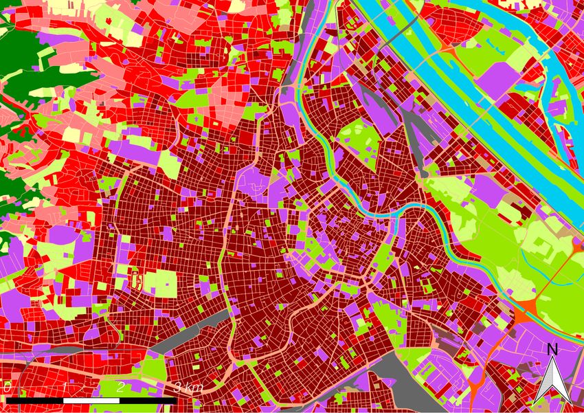
I acknowledge that we are in an existential human-induced climate crisis

   Acknowledgements
                                                            caused by excessive CO2 emissions from a variety of human activities.
                                                             While I recognize that our day-to-day transportation, energy use,
                                                            materialistic consumption, animal-based diets and excessive flying
                                                          impact the climate crisis, individual mitigation alone is no substitute for
                                                                                         policy reform.
                                                                         https://acknowledge-the-climate-crisis.org/

• Joint works with
    •   Paul Kilgarriff and Rémi Lemoy (University of Rouen, FR)
    •   Yufei Wei
    •   Marlène Boura
    •   Kerry Schiel

    • Mirjam Schindler (VUW, NZ)

• Funding: SCALE-IT-UP(400 k€, FNR) Scaling of the Environmental Impacts of Transport and
  Urban Patterns. Luxembourg National Research Fund

 h"ps://showyourstripes.info    Ed Hawkins (University of Reading)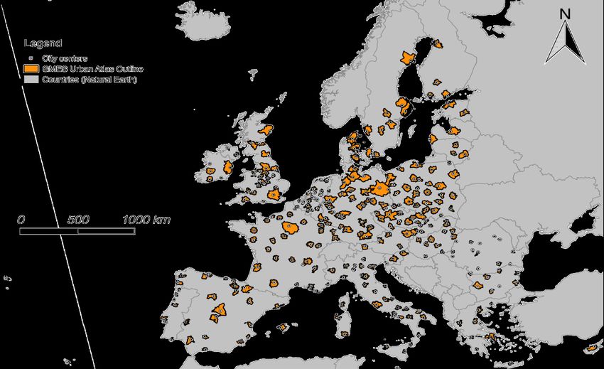
Abstract
We definitely live in an increasingly urban World for half of humanity now lives in cities. Cities provide wealth but also negatively impact the
environment and the health of citizens. Arguably the benefits and costs of cities relate to both their size, in population terms, and their internal
structure, in terms of the relative spatial arrangement of built-up and natural land. Much of urban research focusses on very large cities and
urban cores. Yet 3 urban human out of 4 live in cities of less than 4 million inhabitants (according to the global GHSL dataset). Similarly, 3 out of
4 in a typical (European) city do not live in its core but beyond (using a 7-8km radius to define core for a city like London or Paris). To address
urban sustainability issues and design adaptation policies, these 75% certainly count and, we can argue, also deserve specific attention
because of the relative proximity between urban and non-urban (natural) use that smaller cities and suburban (non-core) areas may permit. In
this respect, it is key to understand how the internal structure of cities, in particular the form and density of built-up areas and the interwoven
green space emerge out of the core up until the fringe. It is also key to understand whether the form of cities, especially density gradients and
the share of urbanised/non-urbanised land change with city size. In this talk we draw lessons from 2 research approaches to urban forms: one
theoretical that uses spatial micro-economic simulations, and one empirical that uses spatially detailed land use datasets. Our theoretical
simulations relate individual behaviour to urban forms while our empirics relate urban forms to city size. Both have in common a radial
perspective to cities, i.e. explicitly or implicitly assuming that the accessibility trade-off to a given centre is a key determinant of locations and
land uses. In both cases, we look at urbanisation and green space structures and at pollution exposure as an example of impact.
3 “urban human” out of 4 live in ci;es of less
than 4 million inhabitants

25% -> Rank 84 ~ 4. 10^6 inhab.
(cumulated: 0.88 billion inhab.)

Author computation from https://ghsl.jrc.ec.europa.eu/datasets.php aggregate urban centers population table

3 “European urban human” out of 4 live out
 of the central core

25% -> within 7 km equivalent of Paris CBD

75% urban popula-on

                               ><

Strong focus on compactness and densifica-on (urban planning) and
              agglomera-on benefits over last 20 years

    “Central city” and “Global city” focus in smart ci-es/urban
              governance/urban economics literature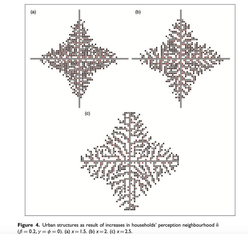
Objectives: Understanding Radial Urban forms
• How urbanisation develops from centre to periphery ?
• Any general law and link with city size?
   • Route 1 : Empirical – statistical trends in land use profiles

• How can different urbanisation forms emerge from simple residential
  choice mechanisms?
   • Route 2: Theoretical – simulations from scratch
Mo;va;ng ques;ons – 1/2 societal/scien;fic
• Are bigger cities better/greener?
   • “as cities get bigger, they get greener in the sense of becoming more
     sustainable” (Batty 2014, p.40) ?
   • Triumph of the city (Glaeser 2012)

• Alternative: What role for smaller cities and for suburbs?
   • Arguably built-up space more closely integrated with natural undeveloped
     land (maybe?) and source of social benefits/environmental effects mitigation?
   • Suburban planet (Keil 2017)

• Which internal structure for a better/greener city given its size?
Motivating questions – 2/2 epistemological

 • A city is more than a single aggregate number as in urban systems theory / and
   geographical economics
 • Liaise intra-urban forms/patterns with aggregate social/environmental
   outcomes, including size

 • Question the definition of a city/urban region
    • E.g. Louf,Barthelemy 2014: whether bigger cities are more green depends on definition

 • Long-run: Integrate dichotomous intra-urban and inter-urban research/theories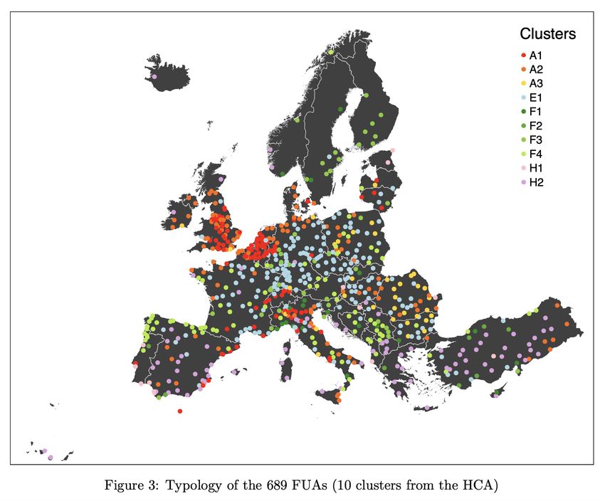
Plan
• Radial/monocentric bias

• Route 1: Empirical research
   • 1.1. Document urbanisaQon profiles in Europe and the World
   • 1.2. Green space gradient /integraQon and ecosystem services

• Route 2: Micro-economic theore-cal simula-ons
   • 2.1. Urban paUerns with endogeneous green space
   • 2.2. Urban paUerns with endogeneous polluQon
Radial perspective – reasonnable “bias”?
• Radial ~
   • One main centre
   • Centre-periphery distance lens
Radial assump;on is empirically acceptable

• Polycentricity emerges when cities grow large (Barthelemy et al.)
  Monocentricity is valid for a very large set of cities. (I am fine with a
  90% relevance ;-))
• Dominance of one center in polycentric systems
• Polycentricity depends on scale, i.e. delineation of cities (see later for
  a resolution):
• Center-periphery interactions are many and add to commuting for
  work/school
Radial assumption is methodologically useful
• Fundamental trade-off between land/housing costs and transportation
  costs

• Dialogue with urban economics where space is 1D
   • Complementarities, falsification tests of theories
   • Clark 1951 negative exp. density , now explored with large datasets

• 1D => Capacity to obtain analytical results mathematically that
   • Complement simulations in 2D space (ABM)
   • Constrain numerical explorations => facilitates exploration of multi-parameters space

• Many planning instruments are implicitly/explicitly radial:
   • green belts, congestion charge, parking policies, housing/land pricing systems,…
Plan
• Radial/monocentric bias

• Route 1: Empirical research
   • 1.1. UrbanisaQon profiles in Europe and the World
   • 1.2. Green space profile /integraQon and ecosystem services

• Route 2: Micro-economic theore-cal simula-ons
   • 2.1. Urban paUerns with endogeneous green space
   • 2.2. Urban paUerns with endogeneous polluQon
Land use data
• Europe:
   •   Urban Atlas 2006 and 2012 (+combined with CORINE Land cover)
   •   N=305 functional urban regions (defined from density and commuting thresholds)
   •   Authors: European Union
   •   Source: https://land.copernicus.eu/

• World
   •   Atlas of Urban Expansion 2016
   •   N=200 select sample
   •   Authors: Angel et al. New York Univ., UN-Habitat, & Lincoln Institute of Land Policy
   •   Source: https://www.lincolninst.edu/publications/other/atlas-urban-expansion-
       2016-edition
Europe : Methods - Europe
1. Radial computation of land use shares (and density) per distance bands
• Vector buffers or Raster-based distances and cross-tabulation
• + Geostats population downscaling for density
2. Stretching of axes as a f(total urban population) to optimize signal/noise
ratio
=> scaling law for internal urban profile !
Ongoing work for EU2012 (combined with CORINE land cover) with total population endogenized.
Methods details and results for EU 2006: Lemoy and Caruso, 2018. Evidence for the homothetic scaling
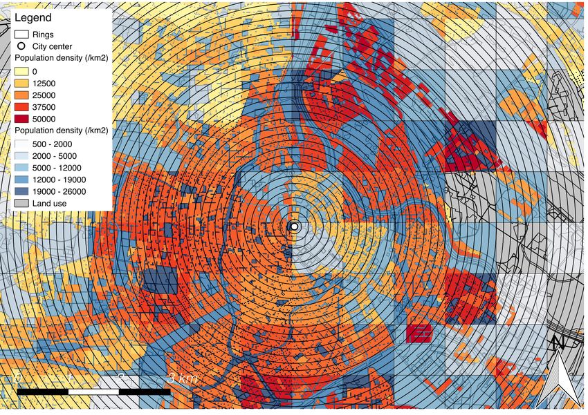
of urban forms. Env. And Planning B.Example Vienna – Urban Atlas
Buffering

CBD =
City halls +
Own corrections

Geostats
Population
downscaling
Ar;ficial Land use profile in Europe (2006)
                                 '
                                                                                         '*'!"

                                !"&
!"#$%&$'( (')* +,- ,.'"- ,/"0

                                                                                                 123 456+('#$5)
                                !"%

                                                                                         '*'!!
                                !"$

                                !"#

                                 !                                                       '!!!!!
                                      !   '!          #!           (!          $!   )!
                                               !"#$%&'( ) $* $+( '(&$() ,-./
Artificial Land profile in Europe - rescaled
'
'*'!"
!"&
Rescaling the
!"#$%&$'( (')* +,- ,.'"- ,/"01
x-axis only, by the
234 567+('#$6)
!"% square root of
'*'!!
population:
!"$ r 0 = r /k,
p
k = N/NLondon
!"#
! '!!!!!
! '! #! (! $! )!
!"#$%&"' '(#)%*$" )+ )," $"*)"- -. /012Artificial Land profile in Europe - rescaled
Finding 1: Strong
central
Rescalingtrendthe(law)
x-axis only, by the
square root of
Finding 2: Square
population:
root
r 0 =isr op-mal
/k,
rescaling
p
k = N/NLondon
Introduction Data and Methods Cities and scaling Conclusion
What is the best rescaling exponent?
’Signal’=
R
hs(r 0 )i2⇡r 0 dr 0
aaa
’Noise’=
R
(s(r 0 ))2⇡r 0 dr 0
aaa
r0 =
r /(N/NLondon )a
Conclusion: cities are homothetic discsArtificial LandAverage
profilelandin
useEurope
Finding 3: constant share
(no drift) at a given
rescaled distance
Great news for defining cities
comparably on a morphological
base!
Let’s compare “core cities” e.g.
defined as 70% of urbanised land
at fringe
or “cities with their sububurbs”
e.g. so that 40 % urbanised land
at fringePopula;on density profile in Europe - rescaled
Finding 1: Strong
Rescaling x- and
central trend (law)
(more y-axes,
dispersedby the
at tail)
cube root of
population :
Finding r 00 =2:r /l, Cube root
is near 00 op-mal
⇢ = ⇢/l,
rescaling of both
axes
Introduction Data and Methods Cities and scaling Conclusion
What l best
is the =exponent?
(N/NLondon )1/3 ’Signal’=
R 00 00
h⇢ (r )i2⇡r 00 dr 00
aaa
’Noise’=
R
(⇢(r 00 ))2⇡r 00 dr 00
aaa
r 00 =
r /(N/NLondon )b
aaa
⇢00 =
⇢/(N/NLondon )bIntroduction Data and Methods Cities and scaling Conclusion
Empirical evidence
Nordbeck to the intuition
(1971)’s homotheties ofgrowth
and allometric Nordbeck 1971
It seems legitimate to claim that all urban areas have the same
form and shape.
In the same way that a vulcano is a volume of dimension 3, so we
may consider population of a tätort [urban area] as a volume with
the same dimensionality. The area of a tätort has the dimension 2.
It follows then that the b-value in the allometric formula A = aP b
ought to be 2/3
Nordbeck, S., 1971. Uban Allometric Growth. Geografiska Annaler. Series B, Human
Geography. 53, 54–67.
Homothetic scaling of urban forms Rémi Lemoy (1), Geoffrey Caruso (1,2)Actually, even with the non-linear model, a large part of the cities are predicted to have more than
Regression
and non-linear es;mate
models of the urban land
100% artificial land in their center, which is impossible. We then try to force this 100% value in the
p
center, and to use a one parameter exponential fit which we call SNL (for simple non-linear model),
follow much more closely the N scaling law found by [1]. Indeed, the e
gradient for any city given its popula;on size
where the only parameter is the characteristic decrease distance lN : sN (r) ⇠ exp( r/lN ). In Table
mple exponential fit for each
1 and on Figure 2,decrease
city. this
There
we comparedistances
are of two ways
the linear
new one-parameter
totodo
fit SNLand
this: to dofitaNLlinear
non-linear
the two-parametermodels are fit
which fitted against tota
or to do a non-linear fitresults
of the
was the most successful rawdisplayed
so far.
are value. in Table 1 (models L and NL, respectively).
LinearTable
(L) 1: Results
log(sof Na (r))
linear⇠ fitlog(a
of theNfitted
) r/l(log)N characteristic distance ⇠ log(lthe
log(lNlN) against 1 ) (log)
+ ↵ total
log N
with
population N , log(lN ) ⇠ ↵ log(N ) + log(l1 ) for the different models: linear fit (L), two-parameter and
↵
Non Linear (NL) sN (r)
one-parameter non-linear fits⇠ aN exp(
(models NL and r/l l
N )respectively) on all cities,
SNL ⇠ l N
N and 1fits on continental
cities only (models NL20 and SNL20, resp.). Note that we exponentiated
imposed to 1 the second fitted coefficient
square error
in this table to obtainThe
is minimised, estimates
but not
the distance ofitssame
the
l1 (and the linear
one:
standard model
the
error) L follow
linear
in meters, fit aofisscaling
which to law
the logarithm
easier with an
interpret. p exponent
ar
quared) relative error, while while the
the estimates
non-linearoffit theminimises
non-linearthe model follow closely
(squared) absolute the N scaling la
We Lsee this all as NL pointing to SNLthe fact thatNL20the non-linear
SNL20 fit is more info
s are illustrated on Figure 1. We observe that⇤⇤⇤the results of the non-linear fit are ⇤⇤⇤
Scaling exponent ↵ one, because
0.310⇤⇤⇤ the non-linear
0.499 fit describes the city center better
0.512 ⇤⇤⇤
0.506 ⇤⇤⇤
0.512 than theroot
Square line
ectations of [1], and also more(0.024) pertinent. Indeed, if we consider first the predicted confirmed
linear fit minimises(0.012)
the square (0.014)
error of the (0.012)
artificial land (0.011)
use shares, while
land in the center, the linear model gives widely dispersed values, ranging from
Exp(constant): l1 (m)the square
124.2⇤⇤⇤ error of 7.64
the⇤⇤⇤logarithm of⇤⇤⇤these shares.
6.23 7.06⇤⇤⇤ As these 6.64shares
⇤⇤⇤ are decrea
200%. We note in particular(45.4) that values (1.32)
above 100%(1.24) are not possible in reality.
from the city center increases, the logarithm(1.15) magnifies the errors further awa
(1.03)
the values given by the non-linear fit are much less dispersed, between 40% and
putting an emphasis on the description of periurban areas. Conversely, the n
values are concentrated around
Observations
the
the expected
302
description of 302100%. Considering
central areas. 302
Thus,
now
the 246the predicted
linear model246 is led astray by sm
R
crease distance lN , the non-linear 0.356 0.847
fit gives ofagain 0.816 0.886 0.897
landless
use dispersed values, which also
2
relative) variations
Linear model on logs in peripheral areas, which the non-linear mo
Note: ⇤⇤⇤
p17 10
Half of the land is urbanised at 5 km from the center for a city of 1 million inhabitants
3.5 1/2
Rescaling= almost sq root (0.512)
Exp(-1)
= 37%
urban land
at 6.64 m for the Singleton CityEU specific? How robust? -> worlwide sample
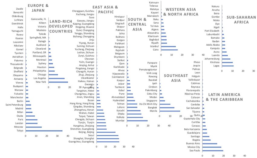
Angel et al, 2016EU specific? How robust? -> worlwide sample
Data and categories from
Angel et al, 2016Artificial Land use profile - Atlas of Urban Expansion
~2014 1.0
0.8
Atlas of Urban Expansion t3
Only few conurba/on polycentricity issues
Legend
Share of artificial LU
0.6
0.4
0.2
0.0
0.0e+00 5.0e+06 1.0e+07 1.5e+07 2.0e+07 2.5e+07 3.0e+07
0 10 20 30 40 50
Distance to the center (km)Artificial Land use profile - Atlas of Urban Expansion
~2014 - Rescaled 1.0
0.8
Atlas of Urban Expansion t3
Legend
Share of artificial LU
0.6
0.4
0.2
0.0
0.0e+00 5.0e+06 1.0e+07 1.5e+07 2.0e+07 2.5e+07 3.0e+07
0 10 20 30 40 50
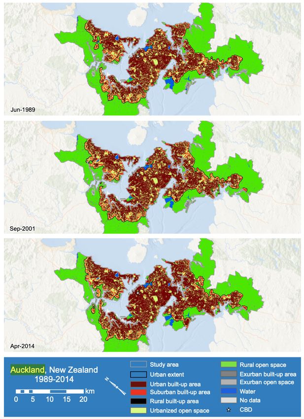
Rescaled distance to the center (km)ArJficial Land use profile - Atlas of Urban Expansion
~2014 – Rescaled (1km smooth) + AUCKLAND, NZ
Atlas of Urban Expansion t3
Legend
1.0
Average profile
+ - 1 sd
0.8
Auckland, NZ
Share of artificial LU
0.6
0.4
0.2
0.0
0.0e+00 5.0e+06 1.0e+07 1.5e+07 2.0e+07 2.5e+07 3.0e+07
0 10 20 30 40 50
Rescaled distance to the center (km)Artificial Land use profile - Atlas of Urban Expansion
~2014 and EU 2012 Urban Atlas compared Atlas of Urban Expansion (2014) and EU Urban Atlas (2012) compared
1.0
Average profile AUE
Finding: Same + - 1 sd
0.8
average profile Average profile EU2012
+ - 1 sd
despite very
Share of artificial LU
0.6
different samples SNL20 fit
and city sizes
0.4
(no significant
difference except for
0.2
smalldistances)
0.0
0 10 20 30 40 50 60 70
Rescaled distance to the center (km)
Mean comparison t-
1.0
test p.value > 0.05From 1D profiles to 2D patterns – An “average” city
Random draw from SNL20 fit Stacking urban land clockwise
100
50
0
−50
−100
−100 −50 0 50 100From 1D profiles to 2D patterns – An “average” city
Stacking urban land clockwise Stacking urban land clockwise
Brussels ParisPlan • Radial/monocentric bias • Route 1: Empirical research • 1.1. Urbanisation profiles in Europe and the World • 1.2. Green space profile /integration and ecosystem services • Route 2: Micro-economic theoretical simulations • 2.1. Urban patterns with endogeneous green space • 2.2. Urban patterns with endogeneous pollution
Green urban space
• Local green space is a strong residen-al choice factor
   • Push towards periphery
   • Source of leapfrogging development (fragmented natural land in periphery)
                                                       see models part 2
   • Source of urban gentrificaQon

• Green space provide
   • leisure and health benefits
   • climate (heat island), polluQon and runoff regulaQon
…. depending on how integrated within the urban fabric (landscape
metrics)
Green urban space – radial profile
Green space − Atlas of Urban Expansion t3
• Theory (Tran and Picard, 2020): skewed inverted U shape of green space in
1.0
equilibrium
• Empirically finding: in line with theory but robustness?… (definition problem?)
0.8
Data: EU Urban Atlas 2006 Data: Atlas of Urban Expansion
Share of artificial LU
0.6
0.4
0.2
0.0
0 10 20 30 40 50
Rescaled distance to the center (km)Green urban space: landscape typology and Ecosystem Services score Ecosystem Services Provision weights Step 1. Link Ecosystem Services with landscape metrics (expansion to Burkhard’s land cover – ES matrix) Step 2. Typology of EU cities Step 3. Ecosystems Services score (weighted sum) per city Boura, Caruso 2020 working paper
Green urban space: landscape typology and
Ecosystem Services score

Boura, Caruso 2020 working paper
Green urban space: Ecosystem Services score
and city size                  Finding: Green space
                                   ES provision decrease
                                   with (log) city size
                                   (even a>er controlling
                                   for urban forest
                                   integraAon types

Boura, Caruso 2020 working paper
Plan • Radial/monocentric bias • Route 1: Empirical research • 1.1. Urbanisation profiles in Europe and the World • 1.2. Green space profile /integration and ecosystem services • Route 2: Micro-economic theoretical simulations • 2.1. Urban patterns with endogeneous green space • 2.2. Urban patterns with endogeneous pollution
How can such general urbanisaJon paUerns
                               emerge?
                         Atlas of Urban Expansion (2014) and EU Urban Atlas (2012) compared
                         1.0

                                                                                              100
                         0.8

                                     What generic process                                                   In what 2D form?
                                     for this profile?
Share of artificial LU

                         0.6

                                                                                              50
                         0.4

                                                                                              0
                         0.2

                                                                                              −50
                         0.0

                               0     10      20        30        40        50      60   70

                                            Rescaled distance to the center (km)              −100
                                                                                                     −100    −50   0    50     100
Micro-economic theory for urban land share profile?
• Urbanisa-on gradients almost completely ignored in urban economics
• Ci#es are en#rely built discs in theory! Only the fringe distance ma8ers.
• The co-existence of developed & undeveloped land at given distance is a puzzle
• (… and how it scales with total popula#on is not a ques#on)
• >< Popula-on density profiles,
• i.e. Density = inverse of housing consump#on, which results from agents trading-
off housing and commu#ng costs (Alonso, 1964)
• Observed scaling of popula#on density profile with popula#on fit theory when
urban land share is controlled for (see Delloye, Caruso, Lemoy, 2019. Alonso and the scaling of
urban profiles. Geographical Analysis)4 “micro” sources for leapfrog/scattered developments
• Dynamic uncertain-es Capozza and Helsley, 1990. The stochas=c city. J. of Urban Economics 28(2): 187-203.
• Thin markets with income heterogeneity Chen, et al., 2017. Market thinness, income sor=ng and
leapfrog development across the urban-rural gradient. Regional Sc. & Urban Economics, 66, pp.213-223.
• Local externali-es: posi-ve effect of green space
• in conQnuous space Cavailhès, et al., 2004. The Periurban City: Why to Live Between the Suburbs and the
Countryside. Regional Sc. & Urban Economics 34, 681–703.
• In 2D discrete space Caruso, et al., 2007. Spa=al configura=ons in a periurban city. A cellular automata-based
microeconomic model. Regional Sc. & Urban Economics , 37(5), pp.542-567; Caruso et al, 2015. Greener and larger
neighbourhoods make ci=es more sustainable! Computers, Env. & Urban Syst, 54, pp.82-94.)
• Local externali-es: nega-ve effect of local pollu-on Schindler and Caruso, 2020. Emerging
urban form–Emerging pollu=on: Modelling endogenous health and environmental effects of traffic on residen=al choice. Env. &
Plan B , 47(3), pp.437-456.Micro-economic 2D simulation model with
green space preference
• CBD and cross-road given at center at t0
• UrbanisaQon develops from successive migraQon
• Endogeneous land market (short-run equilibrium)
• Long-run equilibrium: urbanisaQon stops when
migraQon is no longer beneficial
Residen9al choice:
Radial push-pull (commu9ng vs housing costs)
Local push-pull (socialize vs green) focal func9on
Parameters calibrated to 3 French ciQes ~200 k. inhab.
Caruso et al, 2015Residential choice NO BLACK BOX MODEL
EXPLICIT BEHAVIOUR
Endogeneous rents
Caruso et al, 2015Micro-economic 2D simula;on model with
green space preference
Caruso et al, 2015Poor correspondence to observed average radial profile • Urbanisa(on gradient is too flat 2 promising solu-ons: • Non-linear transport costs • Differen-ated neighbourhood size for the local effects (green space valued at larger distance from home than local density spillovers)
Generic norma;ve lessons from changing
         parameters/changing parameters
         • Example: increasing neighourhood size, i.e. facilitating trips at no cost
           to local green
         • => different spatial arrangement of built and green space
         • => welfare and sustainability gains for a given population

Caruso et al, 2015
Plan • Radial/monocentric bias • Route 1: Empirical research • 1.1. Urbanisation profiles in Europe and the World • 1.2. Green space profile /integration and ecosystem services • Route 2: Micro-economic theoretical simulations • 2.1. Urban patterns with endogeneous green space • 2.2. Urban patterns with endogeneous pollution
Micro-economic 2D simula;on model with
   traffic pollu;on
        • No explicit preference for green space
        • Avoidance of local traffic pollution
        • Sprawl and scatteredness increase with
             • increasing pollution awareness
             • Increasing size of pollution perception
               neighbourhood
        • Resulting radial profile of pollution

Schindler and Caruso, 2020
Concluding remarks • Homothetic radial profiles: large cities are no exceptional urban forms but… larger objects • Local environmental effects (impact not divisible per capita) worsen with city size • But the spatial arrangement of built and non-built/green space seem to be key under the constraint of a given radial profile • Suggestion/wish: shift away some urban research focus from large and core cities’ smartness to smaller cities and suburbs, which may be easier to ‘retrofit’ with nature
Thank you for your attention!
       geoffrey.caruso@uni.lu
You can also read


