State of California THE NATURAL RESOURCES AGENCY - Wilmers Lab
←
→
Page content transcription
If your browser does not render page correctly, please read the page content below
State of California
THE NATURAL RESOURCES AGENCY
California Department of Fish and Wildlife

FINAL REPORT SISKIYOU DEER-MOUNTAIN LION STUDY (2015-2020)

HEIKO U. WITTMER1, BOGDAN CRISTESCU2, DEREK B. SPITZ2, ANNA NISI2 &
CHRISTOPHER C. WILMERS2
1
 School of Biological Sciences, Victoria University of Wellington, PO Box 600,
Wellington, 6140 New Zealand (heiko.wittmer@vuw.ac.nz)
2
 Environmental Studies Department, 1156 High Street, University of California, Santa
Cruz, California 95064, USA

Suggested Citation:

Wittmer, H.U., Cristescu, B., Spitz, D.B., Nisi, A. & Wilmers, C.C. (2021). Final report
Siskiyou deer-mountain lion study (2015-2020). Report to the California Department of
Fish and Wildlife. 71pp.

Disclaimers: The findings and conclusions in this report are those of the authors and do
not necessarily represent the views of the California Department of Fish and Wildlife or
the University of California Santa Cruz. The use of trade names of commercial products
in this report does not constitute endorsement or recommendation for use by the
government of the State of California or the University of California system.
FINAL REPORT SISKIYOU DEER-MOUNTAIN LION STUDY (2015-2020)

INTRODUCTION

Mule (Odocoileus hemionus) and black-tailed deer (O. h. columbianus) have long
experienced pronounced population fluctuations across their distribution in western
North America inclusive of California (Leopold et al. 1947). The underlying mechanisms
for the observed short and long-term fluctuations are complex and remain inadequately
understood (e.g., Ballard et al. 2001, Pierce et al. 2012, Forrester & Wittmer 2013,
Monteith et al. 2014). At high population densities, mule and black-tailed deer appear
mostly limited by forage availability and weather with the effect of predation considered
largely compensatory (Laundre et al. 2006, Hurley et al. 2011, Pierce et al. 2012).
However, compared to many other ungulates, mule and black-tailed deer experience
lower and more variable survival of fawns particularly over the initial 6-months period
following births (Gaillard et al. 2000, Forrester & Wittmer 2013). The most commonly
reported cause of fawn mortality across their ranges is predation from a diverse guild of
mammalian predators including black bears (Ursus americanus), coyotes (Canis
latrans), and mountain lions (Puma concolor). Relatively high fecundity rates typical of
Odocoileus apparently enable them to compensate for low fawn survival over longer
time frames (Forrester & Wittmer 2013). Recent observations of high predation on both
fawns and adult deer, particularly, but not exclusively, in systems that have experienced
pronounced changes in predator or alternative prey populations (e.g., Robinson et al.
2002, Cooley et al. 2008, Marescot et al. 2015), have reignited interest in understanding
the overall impact of top-down versus bottom-up effects on deer population dynamics.

Two recent changes to our understanding of how direct and indirect interactions
between two predator species as well as between predator and their prey species may
affect deer populations warrant further investigation. First, black bears have long been
known to be an important predator of juvenile cervids including mule and black-tailed
deer (e.g., Griffen et al. 2011, Forrester & Wittmer 2019). Recent research, however,
has also shown how effective black bears are at usurping deer killed by mountain lions
(i.e., kleptoparasitism; Allen et al. 2015a, Elbroch et al. 2015), the primary predator of
adult deer across much of their range. For example, in the Mendocino National Forest in
northern California, black bears detected 77.2% of deer killed by mountain lions that
researchers monitored with cameras (Elbroch et al. 2015) causing the rapid
displacement of mountain lions from the majority of these kills. The resulting energetic
costs associated with lost feeding opportunities (Elbroch et al. 2014) apparently forced
mountain lions to kill adult black-tailed deer, the only ungulate prey species in the
system, at rates higher than those observed across the mountain lion’s range (Cristescu
et al. 2020, Allen et al. 2021). The combined effect of high predation of fawns including
from black bears (Forrester & Wittmer 2019) and high predation rates on adult deer
from mountain lions (Marescot et al. 2015, Allen et al. 2015b) resulted in a rapid, short-
term decline (population growth rate (!) based on vital rates estimated from a 5-year
monitoring study = 0.82) of the local black-tailed deer population (Marescot et al. 2015).
Note though that black-tailed deer in the Mendocino National Forest occurred at high
densities on summer range at the time of the observed decline (Lounsberry et al. 2015).

                                                                                        2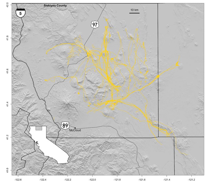
Second, the recovery of some apex carnivores such as wolves (Canis lupus) in the
western United States not only adds another predator of deer in some ecosystems but
further increases the complexity of predator-prey interactions through potential direct
and indirect effects on subordinate competitors of wolves including mountain lions
(Elbroch et al. 2020). Understanding the effect of complex predator interactions,
including those mentioned above, on prey populations requires research projects that
simultaneously monitor both predators and their prey (e.g., Pierce et al. 2012, Marescot
et al. 2015).

Mule and black-tailed deer are the most widespread and abundant ungulates in the
State of California, providing recreational opportunities including hunting. The public has
raised concerns about the apparent decline of deer populations in several areas of the
State (e.g., Siskiyou and Mendocino counties) as well as the lack of research aimed at
understanding the underlying causes for the decline. This provided the impetus for
developing and funding a range of research and monitoring projects aimed at providing
the California Department of Fish and Wildlife (CDFW) with current data needed to
inform deer management decisions. Studies aimed at understanding the underlying
causes for fluctuations or possible directional changes in deer populations rely on
detailed multi-year studies of telemetered individuals. Such studies provide information
including age-specific vital rates, causes of mortality, and their combined effect on deer
population growth. They can also help understand movement patterns and resulting
population structure and help quantify the link between habitat use and selection and
overall population performance. Studies of telemetered deer in California are currently
being expanded to be representative of the diversity of ecosystems in the State, and
continued data collection is crucial for developing and updating effective deer
management and conservation plans (e.g., Pierce et al. 2012, Monteith et al. 2014,
Forrester et al. 2015, Marescot et al. 2015, Bose et al. 2017, 2018).

In northern California’s CDFW Region 1, declining hunter harvests of deer, apparent
deer population declines, and a lack of information about factors affecting deer
populations have long generated considerable interest from the public and resource
management agencies. In 2010, the Siskiyou County Board of Supervisors thus passed
a resolution to actively encourage, develop, and help implement cooperative strategies
and projects geared toward research, restoration, and sustainability of abundant,
healthy deer conservation units in the Region. The Siskiyou Deer-Mountain Lion Study,
a collaboration between the CDFW and the University of California Santa Cruz (UCSC),
is ultimately an outcome of this resolution. Deer captures for the project started in 2015
with UCSC researchers taking over study responsibilities upon execution of the contract
agreement on 15 June 2016 (Agreement Number P1580031). The Siskiyou Deer-
Mountain Lion Study had the following specific objectives:

1. Identify specific study area(s) and study sites in agreement with the California
Department of Fish & Wildlife.

2. Estimate deer population size, composition, and changes in abundance using fecal
DNA mark-resight methods.

                                                                                         3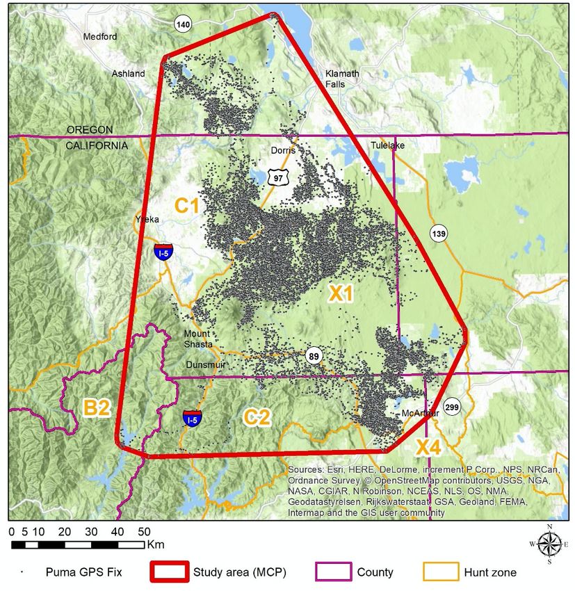
3. Assess factors influencing deer population growth

     a) Estimate deer population change within project study sites using matrix
     modelling approaches that incorporate estimates of annual fawn and adult female
     survival, and age class-specific pregnancy rates and litter sizes.

     b) Evaluate the potential effect of conception date on fawn survival and
     recruitment.

     c) Investigate the hypothesis that post-season buck ratios influence conception
     dates.

     d) Determine the relationship between age and body condition of adult female deer
     and their productivity.

     e) Investigate relationships between habitat quality/quantity and productivity of
     female deer.

     f) Estimate the occupancy and/or abundance of carnivores including mountain
     lions, black bears, coyotes, and bobcats within representative sites.

     g) Determine rates of predation as a function of deer sex and age classes and its
     potential influence on deer population growth.

     h) Assess the diets of mountain lions in the study area and their rates of predation
     on deer.

     i) Test the hypothesis that competition with other carnivores (e.g., black bears)
     increases predation rates on deer by mountain lions.

4. General deer ecology

     a) Identify the diet composition and seasonal changes in foraging strategies of
     deer.

     b) Identify and describe characteristics of core reproductive areas, migration
     corridors, and winter ranges of radio-collared deer.

This report summarizes current outcomes of the study using data collected over the
time period from March 2015 until the end of fieldwork in June 2020.

STUDY AREA

The study area is located in northern California. The area primarily falls within the X1
and C1 hunting zones and was selected by the CDFW. The study area is likely part of

                                                                                           4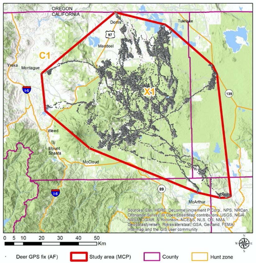
an introgression zone between black-tailed deer primarily to the west and mule deer
primarily to the east and from here onwards we will refer to them simply as “deer”. We
defined overall study area boundaries post-hoc based-on GPS locations of all collared
deer and mountain lions. A minimum convex polygon (MCP) encompassing all deer
locations extended over 6,702 km2 (Fig. 1A) and covered four counties: Siskiyou,
Modoc, Shasta, and Lassen. The corresponding MCP encompassing all mountain lion
locations was much larger (15,335 km2) and included areas in southern Oregon to the
north and Shasta Lake to the south (Fig. 1B).

                                                                                         5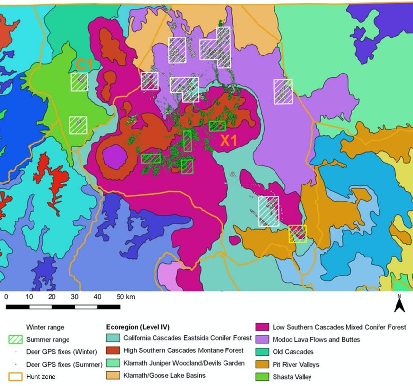
Fig. 1. (A) Siskiyou deer study area as delineated by a minimum convex polygon (MCP) based
on GPS location data from 81 adult female deer monitored between 2015-2020. (B) Siskiyou
mountain lion study area MCP based on GPS location data from 14 mountain lions monitored
between 2017-2020.

The terrain and topography of the study area are extremely diverse. The western parts
of the study area encompass Mount Shasta (4,322 m/14,179 ft) and thus included the
southern end of the Cascade Range. Topography in the southern Cascade Range is
dominated by complex and steep terrain. Where topography is less pronounced,
remaining cones of extinct volcanoes add terrain complexity. The north-eastern parts of
the study area are dominated by plateaus that range in elevation from approximately
1,350-2,000 m or 4,430-6,560 ft. Plateau topography is formed by volcanic activities and
included Lava Beds National Monument. Both elevations and topography are less
pronounced in southern and north-eastern parts of the study area. The climate in the
study area varies locally but is generally characterized by dry and warm summers and
cool and, in some places, wet winters. Annual precipitation ranges from approximately
250 mm in the northeast to 1,000 mm in the south around Shasta Lake. Most of the
precipitation falls as snow in winter, particularly at higher elevations. Significant snow
accumulation on higher peaks including Mount Shasta ensures the gradual release of

                                                                                             6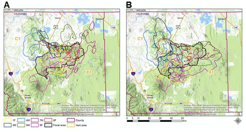
moisture well into the dry summers. Nevertheless, surface water often dries up during
the hottest months of the year.

Landownership included public (state and federal) and private lands. The majority of the
study area fell within 3 National Forests: Shasta-Trinity, Klamath, and Modoc National
Forests. Past and current logging operations in these National Forests have resulted in
a mosaic of unevenly aged forest stands including large clear-cuts that are sometimes
being actively replanted by logging operators. The past logging history is extensively
summarized in the McCloud Flats Deer Plan (California Department of Fish & Game
1983). Some forest stands are privately owned and operated. Agricultural activities on
private lands included limited alfalfa production relying on artificial watering practices
and low-intensity livestock production, particularly cattle. Several major highways
dissected the study area. Notable were I-5 and HWY 97 to the west and north-west, and
HWY 89 to the south. Train tracks following a north to south direction were also
dissecting the study area. The National Forests are serviced by a network of well-
maintained forest roads, both paved and unpaved. However, with the exception of traffic
associated with logging operations, traffic on these forest roads was almost exclusively
limited to tourism in the summer months and the fall hunting season. Only a few, small
settlements can be found within and in the vicinity of the study area, the largest being
the town of Mount Shasta with approximately 3,300 inhabitants.

The study area encompasses several Level IV ecoregions including (from west to east):
Shasta Valley, High Southern Cascades Montane Forest, Low Southern Cascades
Mixed Conifer Forest, Modoc Lava Flows and Buttes, California Cascades Eastside
Conifer Forest, and Pit River Valleys (Environmental Protection Agency 2012). Despite
much of the soils consisting of weathered volcanic rocks with limited suitability for
agriculture, the varied terrain and localized climate and soil moisture levels result in a
very diverse plant community, particularly of shrubs. Based on the CALVEG landcover
type classification, eastern ranges are predominantly juniper (Juniperus spp.) and
sagebrush (Artemisia spp.), with juniper also widespread in the west. Across the
remainder of the study area, lower elevations are dominated by bitterbrush (Purshia
tridentata) in the north, ponderosa pine (Pinus ponderosa), and mixed shrub and
conifers in the south and west. Higher elevations supported mixed montane shrubs,
mixed conifer, and fir (Abies spp.) forests.

Deer are the most abundant and widespread native ungulate across the study area.
Other native ungulates include elk (Cervus canadensis) and, localized, pronghorn
(Antilocapra americana). Cattle were grazed on both public and private lands and some
feral horses were present in the central north-eastern part of the X1 deer hunt zone.
Mountain lions, black bears, coyotes, and bobcat (Lynx rufus) were present at
presumably varying densities across the study area. One wolf pair was known to be
present and reproduce in the study area at the onset of the project in 2015 but failed to
establish a permanent population and wolves were considered functionally absent
between 2016 and 2020.

                                                                                         7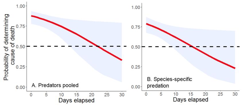
METHODS

STUDY SITES

Based on historical information, we expected deer in the study area to be migratory
(California Department of Fish & Game 1983). We used input from CDFW and GPS
location data from collared adult female deer to help select initial study sites within the
study area. Specifically, we used initial GPS location data for female deer captured in
the winter of 2015 by the CDFW (see adult deer captures below) to scout and
subsequently select suitable sites for capturing deer fawns on summer ranges in 2016.
We then coordinated with the CDFW and continued adult deer captures on both
summer and winter ranges in subsequent years and used all available deer location
data until 2017 (i.e., GPS location data from adult females, VHF location data from
fawns) to identify and delineate potential deer winter ranges. These ranges should not
be considered distinct (i.e., deer are likely continuously distributed across the landscape
albeit at varying densities) as they are necessarily only a representation of areas used
by our sample of deer rather than the deer population per se. Also, the primary purpose
of delineating these potential summer and winter ranges was to develop and conduct
vegetation surveys over an area we also attempted to estimate deer densities for (see
deer population density below) and thus allow us to assess the importance of bottom-up
(i.e., forage related) impacts on deer.

FAWN CAPTURES & MONITORING

We conducted fawn captures under a scientific collection permit issued by the California
Department of Fish & Wildlife (SC10859). All fawn capture and handling procedures
were further approved by an Institutional Animal Care and Use Committee at the
University of California, Santa Cruz (protocols Wilmc1509 & Wilmc1811) and adhered to
guidelines established by the American Society of Mammalogists (Sikes et al. 2016).

We captured fawns from June 16th onwards during our 2016 pilot study immediately
after the contract had been executed (n = 4). Between 2017 and 2019, we captured
fawns from June 1st onwards until early July (n = 141) using 3 different methods. First,
we drove along forest roads and used handheld spotlights on both sides of the vehicle
to locate fawns during the night. Second, we opportunistically captured fawns we
encountered while driving during daylight hours. Finally, we scanned meadows and
forest habitats during both day (binoculars) and night (spotlights) for post-parturition
females and walked in to locate nearby hidden fawns if we deemed doe behavior
suspicious (e.g., hesitation or unwillingness to move away despite being approached,
frequent scanning of the same location). We captured fawns either by hand or with
handheld nets, and sometimes after a brief chase. Capture personnel wore new latex
gloves for each capture to minimize scent contamination. Once captured, we transferred
fawns into pillowcases where they could be more easily handled. Handling of fawns
included recording their sex, weight, and then fitting all individuals with small colored
and numbered plastic ID ear tags. We also recorded the state and dryness of the
umbilical cord and measured hoof growth lines with calipers (Sams et al. 1996) to

                                                                                          8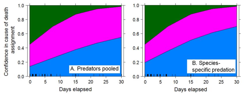
estimate the approximate fawn age at capture. Finally, we attached very high frequency
(VHF) motion-sensitive radio collars (Vectronic Aerospace, Germany) with expandable
neckbands that were purpose-designed for fawns. Collars were programmed to switch
to a mortality signal if they remained stationary for > 4 hours. Based on factory
programming (VHF signals were active from 6 am until 10 pm), we estimated that
batteries should last for up to 2 years. Based on 129 captures for which processing
times were recorded, capture processing ranged from 5 - 20 minutes and averaged
approximately 11 minutes. Once collared, fawns were released at their capture sites.
We limited handling procedures for fawns that struggled or vocalized excessively to only
attaching the VHF collar. This was to avoid capture related injuries, to minimize stress,
and to reduce the likelihood of drawing in potential predators of fawns. Note that we
returned to the capture location over the following 24 hours to install a remote camera
(see information on predator monitoring below).

We monitored the status of fawns (survival and general location) daily from capture until
early September using ground-based telemetry. We reduced monitoring efforts to 1-4
times per month until fawns turned 1 year old in June the following year. Such changes
in monitoring frequency are common (e.g., Marescot et al. 2015) as daily monitoring is
thought to facilitate the assessment of causes of mortality when fawns are small.

YEARLING DEER MONITORING

No 1-year-old deer (yearlings) were captured and collared during the study. However,
the approximately 2-year initial battery life expectancy of fawn collars allowed us to
continue monitoring surviving fawns as yearlings and until they transitioned into the
adult age class on their second birthday. Small batteries powering fawn collars reduced
the range of their VHF signal making ground-based relocation efforts challenging.
Nevertheless, monitoring of yearlings was attempted at least once per month.

ADULT DEER CAPTURES, MONITORING, AND MOVEMENT STRATEGIES

All captures of adult female deer ≥ 2-years-old were the responsibility of the CDFW and
followed an internally approved capture plan. Captures were initially conducted by
helicopter using netguns in March 2015 (n = 25). All captured deer in 2015 were flown
to a central processing site where they were restrained with leg hobbles. At the
processing site, deer were weighed and provisionally aged based on tooth wear and
eruption patterns. Twenty-one deer were administered lidocaine (0.5 cc of a 2%
solution) prior to also having a tooth extracted for age determination using cementum
annuli methods but all samples that year were retained by CDFW staff and
unfortunately were lost prior to submission to the contracted lab for processing. Blood
samples were taken including to test for pregnancy based on progesterone levels and
an ultrasound was used to confirm pregnancy and record the number of fetuses in uteri.
Deer received a number of prophylactic treatments at varying doses including Penicillin
(3-4 cc), Cloxacillin (1 cc), Vital E (3-5 cc), and MuSe (1 cc), all administered
subcutaneously. Finally, the body conditions of all deer were assessed at up to four
body parts. Assigned body condition scores (BCS) ranged from 1 (very poor) to 5

                                                                                        9
(excellent) and increased in 0.5 increments. We report BCS assessed at the base of the
tail (preferred) or the pelvis (if no value was recorded for the base of the tail) as these
were likely most closely aligned with scores assigned at deer captures in subsequent
years (see below). All deer then received an individually numbered ear tag ID and most
were fitted with two collars. The first collar, a GPS “lifetime” collar (Survey Globalstar,
Vectronic Aerospace, Germany) with satlink and VHF capabilities, recorded locations
once every 2 weeks and was intended to remain on the animal for its remaining life. A
second, satellite-enabled GPS collar (Vertex Plus Iridium, Vectronic Aerospace,
Germany) recorded locations every 1 hour and was programmed to automatically drop
off after 1 year. GPS collars were also programmed to send mortality notices via
satellite if a collar remained stationary for > 4 hours. Combined, collar weights were
below 3% of body weights of adult deer. Deer were either released at the processing
site or returned to the vicinity of their original capture locations.
In subsequent years, adult female deer were searched for by driving along forest roads
and captured using a tranquilizer dart delivered with a dart gun from the vehicle and
sometimes after stepping outside the vehicle for a brief stalk. This allowed for a more
targeted collaring of adult deer in areas where we also captured fawns (see above).
Captures occurred in July-August of 2016 (n = 17), August-September 2017 (n = 11
including 2 recaptures of previously collared individuals), and both March (n = 16) and
August-September (n = 19) of 2018. Deer were anesthetized using a Telazol/Xylazine
combination. Teeth samples were collected for age determination using cement-annuli
methods (Matson’s Laboratory LLC, Missoula, MT, USA) during 17 captures in 2016
and 33 captures in 2018. An ultrasound was used for females captured in March 2018
to determine the number of fetuses in uteri. Body condition assessments slightly differed
from those in 2015. Specifically, assessment was based on a modified rump fat body
condition score (rBCS) that ranges from 1 (very poor) to 5 (excellent) (Gerhart et al.
1996, Cook et al. 2010) which is the more commonly used BCS in CDFW deer research
projects. Other handling procedures followed those described above. All deer were
fitted with one Vertex Plus Iridium GPS collar programmed to drop off after 1-1.8 years,
except deer captured in March 2018 that were fitted with one Survey Globalstar GPS
collar. Vertex collars were programmed to record locations every 1 hour (2016 captures)
or every 2 hours (2017 and 2018 captures). Survey collars were programmed to acquire
one location every 13 hours, which was the most intensive fix rate possible with this
collar model. All deer were reversed using Tolazoline and released at their capture
location.
Note that Survey Globalstar GPS collars functioned for much shorter time periods than
anticipated. However, the associated VHF transmitters in these collars allowed us to
continue monitoring the status of adult female deer once every month using ground-
based monitoring described for fawns and yearlings above.
We quantified movement strategies of GPS collared deer based on net squared
displacement (the square of the distance between the starting point and each
subsequent point; NSD) of individual deer tracks using the R package MigrateR 1.1.0
(Spitz et al. 2017). We fitted the NSD of each yearly track to models representing 1)
10residency, 2) nomadism, 3) dispersal, 4) migration, 5) mixed migration, and 6) multi-
range migration (Spitz et al. unpublished manuscript). We compared the fit of these
models to the NSD of each track using Akaike Information Criterion (AIC; Burnham &
Anderson 2002) and selected the best supported movement classification for each deer.
This approach allowed us to determine migration distances between summer (fawning)
and winter ranges. Furthermore, it allowed us to visualize potentially important
movement routes and thus identify possible interactions of collared deer with highways
in the study area.
DEER CAUSE OF MORTALITY ASSESSMENTS
Once UCSC personnel assumed responsibilities for monitoring both fawns and adult
deer from June 2016 onwards, causes of mortalities were investigated and assigned
based on a purpose developed assessment method. A detailed protocol describing our
methods will be submitted for peer-review to a scientific journal. The protocol describes
the field assessment, all evidence collected at the mortality site, and how evidence was
used to determine the cause of mortality. Our framework also describes a practical
method for assigning a confidence level (low, medium, high) to cause of mortality
assessments in the field. We report causes of mortality in this report including levels of
confidence but refer to Cristescu et al. (unpublished manuscript) for further details
regarding our methodology.
DEER VITAL RATES
Data collected during captures and the subsequent monitoring of collared individuals
allowed us to estimate the following vital rates for deer.
a) Pregnancy rates: Estimated from data collected for 25 females captured in March
2015 and 16 females captured in March 2018 (yes or no). Annual pregnancy rates are
derived by dividing the total number of individuals confirmed pregnant in a given year by
the total number of females assessed the same year. From these annual values we
then determined the mean annual pregnancy rate for our deer sample.
b) Number fetuses per pregnant female: Estimated from ultrasound data collected for
pregnant adult females captured in March 2015 (n = 24) and March 2018 (n = 15). From
these annual values we determined the mean number of fetuses/female for our deer
sample.
c) Fawn survival: We estimated monthly fawn survival from the monitoring history of
telemetered individuals using a staggered-entry design for the Kaplan-Meier estimator
(Pollock et al. 1989). All fawns entered the survival analysis in the months they were
captured. We censored individuals in the month when we no longer were able to
confirm their status. We used the estimated date of mortality from our detailed mortality
site investigations to allocate a month to all fawns we confirmed to have died during the
study. We then converted monthly survival estimates into yearly survival estimates and
estimated the overall mean annual survival rate of fawns (±SE) from these yearly
11estimates. We did not estimate survival rates of female and male fawns separately as
our annual sample sizes were not large enough.
d) Yearling survival: We estimated the survival rate of yearlings from the monitoring
history of telemetered individuals using a staggered-entry design for the Kaplan-Meier
estimator (Pollock et al. 1989) as outlined for fawns above. However, due to low yearly
sample sizes, we pooled the monitoring histories of all individuals (females and males)
across all years into one monitoring period with 12 monthly intervals. Even with pooling,
the average number of yearlings monitored per month was only 11.58 (±8.11 SD) with
monthly sample sizes particularly low from December onwards due to issues associated
with battery life of collars and difficulties tracking movements particularly those of
dispersing male yearlings. While pooling was necessary due to low sample sizes, it may
have resulted in slightly biased (i.e., low) survival estimates for female yearlings due to
the likely elevated risk of mortality of male yearlings during dispersal.
e) Adult female survival: We estimated the survival rate of adult females ≥ 2-years-old
as outlined for fawns above as we deemed average monthly sample sizes of collared
adult females of 26.33 (±10.53 SD) females/month large enough to result in unbiased
estimates. Due to the limited information collected on age of our sample of collared
adult females, we did not attempt to investigate possible reduced survival of senescent
individuals.
DEER POPULATION GROWTH
We used a post-breeding Lefkovitch projection matrix (Caswell 2001) to estimate the
population growth rate (!). As mule and black-tailed deer are polygynous, we built a
female only matrix with 3 stages: fawns, yearling, and adults. We assumed deer to first
reproduce as 2-year-olds (Monteith et al. 2014). As none of the females assessed for
pregnancy in our study were classified as yearlings, we used pregnancy rates for mule
deer provided in Monteith et al. (2014) to adjust our data collected for adult females
accordingly. Specifically, data in Monteith et al. (2014) suggested that the pregnancy
rate of a sample of 22 yearlings was 69.4% of the pregnancy rate of a sample of 803
adult females (i.e., 0.68 versus 0.98). We also adjusted the number of fetuses to reflect
a 50:50 sex ratio at birth. Combined, these adjustments allowed us to calculate stage-
specific reproductive rates (r) as the product of pregnancy rates, mean number of
fetuses, fawn sex ratio, and stage-specific survival. In the absence of precise age
estimates based on cementum annuli for all collared females and resulting small sample
sizes, we refrained from adding a “senescent” stage to our projection matrix despite
research in deer and other ungulates showing declines in both survival and reproductive
rates with increasing age (Gaillard et al. 2000, Marescot et al. 2015). Our estimates of !
may thus be slightly biased high. Using our vital rate estimates, we parameterized the
following matrix
0 &! &"
" = $'# 0 0 (,
0 '! '"
12where ' denotes stage-specific survival probabilities for fawns (f), yearlings (y) and
adult females (a), and r denotes stage-specific reproductive rates for yearlings (y) and
adults (a).
We used a simulation approach to estimate ! and to account for uncertainty in estimates
of vital rates. Specifically, we ran 1,000 iterations of our matrix calculations in which
age-specific survival probabilities and pregnancy rates were drawn from a beta
distribution based on their respective means and standard errors (survival rates) or
standard deviations (pregnancy rates). Note that in the absence of actual data, we used
the standard deviation derived from pregnancy data of adult females for our adjusted
pregnancy rates of yearlings. For each iteration, we also drew the expected number of
fetuses per female from a gamma distribution based on the respective parameter mean
and standard deviation. We then derived estimates of lambda from the dominant
eigenvalues of the 1,000 simulated matrices and determined 95% confidence intervals
based on the percentile method. Finally, we conducted sensitivity and elasticity
analyses using the vitalsens function in the R package popbio (Stubben and Milligan
2007) to understand absolute and relative contributions of underlying vital rates as well
as matrix elements to projected deer population growth.
DEER POPULATION DENSITY
a) Summer: Starting at the end of July 2017, we established pellet transects on 4
summer (fawning) ranges to estimate deer densities based on DNA capture-mark-
recapture methods (Lounsberry et al. 2015). We established 6 transects per fawning
area for a total of 24 pellet transects. Including the initial setup, each transect was
sampled 6 times with on average 9 days (range = 7-10) between sampling events. Deer
pellets were collected until September 2017 following a protocol outlined in Brazeal et
al. (2017). In total, we collected 960 pellet samples (4-6 pellets per pellet group
encountered), of which 402 were “fresh” and 558 “not fresh” according to pre-
established criteria. The samples were stored in ethanol and transferred for DNA
extraction to Dr. Ben Sack’s lab at the University of California, Davis. In total, 261
samples (of 520 chosen from the 2017 samples) were successfully genotyped for
summer ranges. This resulted in 142 individual deer being identified (average capture
rate = 1.84).
b) Winter: During January-April 2019, we established a total of 28 pellet transects to
estimate deer densities on 8 winter ranges. Transect setup and deer pellet collection
followed published protocols described for summer ranges above and each transect
was sampled 5 times with on average 9 days (range = 7-12) between sampling events.
Pellet collection was completed in mid-April 2019. In total we collected 1,072 pellet
samples (4-6 pellets per sample). The samples were again stored in ethanol and
transferred to Dr. Ben Sack’s lab at the University of California, Davis, for DNA
extraction. In total, 672 samples (of 1072 chosen from the 2019 samples) were
successfully genotyped for winter ranges. This resulted in 419 individual deer being
identified (average capture rate = 1.60).
13In addition to pellet collection, we deployed remote cameras in the same areas as the
transects to obtain information on deer age class and relative group size on winter
ranges (Furnas et al. 2018). The camera data can be used to refine statistical modelling
of pellet-based deer density estimates as it helps understand the age- and sex
composition of deer in the vicinity of transects. While cameras were not specifically
established on pellet transects on summer ranges, comparable data was collected with
cameras deployed at fawn capture locations on the respective ranges (see predator
monitoring below).
DNA genotyping data was provided to Dr. Brett Furnas (CDFW) who used a SECR based
approach to estimate age- and sex-specific deer densities on both summer and winter
ranges in the study area.
DEER DIET
a) Summer: From the end of July until September 2017, we collected deer pellet
samples along the 24 pellet transects we established for DNA-based deer density
estimation (6 transects in each of our 4 fawning areas). We collected two pellets from
each deer pellet group encountered that contained non-degraded/non-partially
decomposed pellets. Samples were pooled across transects for each fawning area. We
stored samples in dry bags for microhistology analysis of deer diet by a suitable lab.
b) Winter: During January-April 2019, we collected deer pellet samples along the 28
pellet transects we established for DNA-based deer density estimation on 8 winter
ranges. We collected two pellets from each deer pellet group encountered that
contained non-degraded/non-partially decomposed pellets. Samples were pooled
across transects for each sampling area (winter range). We stored samples in dry bags
for microhistology analysis of deer diet by a suitable lab.
All deer diet samples were provided to the only remaining lab in the US who still conducts
microhistology analyses from pellets, but samples have not been processed at the time of
writing. External funding has been secured for the analysis to be completed.
While deer diet estimates from pellets have not yet been processed, we can provide a
detailed list of plant species that, combined, contribute significantly to the diet of deer in
the study area. The list is based on signs of deer browsing recorded during our
intensive vegetation surveys.
DEER FORAGE AVAILABILITY & QUALITY
During July-October 2018, we carried out intensive habitat surveys on summer ranges
to estimate deer forage availability. Surveys were designed to quantify plant species
composition, percentage cover, and biomass using the line intercept and yield rank
14methods (summarized in Higgins et al. 2012). Surveys covered our 4 focal summer
(fawning) ranges (Asperin Butte, Buck Mountain, Fons Butte, Red Hill). During
February-April 2020, we also carried out intensive habitat surveys on deer winter ranges
to estimate forage availability. Surveys occurred on 8 focal winter range areas (Day
Bench, Lake Shastina, Montague, Mount Dome, Mount Hebron, Sheep-Mahogany
Mountain, Tionesta, and Wildhorse Mountain). Each line intercept was 100 m long and
oriented on a random cardinal direction. Any vegetation that came into contact with an
intercept pole, or its projection 1.8 m above ground level was considered intercepted.
The 1.8 m mark represents the approximate maximum height of deer foraging, limiting
sampling efforts to available food. Ferns on both summer and winter ranges, and
conifers other than firs on summer ranges were not recorded when encountered due to
either no or low expected utilization by deer.
We recorded plant species intercepted at 1 m marks along the transect to the finest
taxonomic level possible and measured the plant specimen’s length and width. In
summer, forbs were identified to species or genus levels, whereas graminoids were
classified as grasses, sedges, or rushes. In winter, herbaceous vegetation was pooled
as either forb or graminoid because of difficulties in identification due to the dry state of
the vegetation. To estimate woody forage biomass available to deer, we laid out 5 x (1
m x 1 m) quadrats at equal intervals along each transect and counted all palatable live
twigs of woody plants within the quadrats. Counts included all live palatable annual
growth twigs up to 1.8 m high to reflect browse material available to deer. Palatability
was determined based on shrub species-specific browse diameters, that we calculated
based on measuring the diameter at point of browse for 100-200 twigs from specimens
we measured at randomly sampled locations prior to laying out the line intercept
transects. To estimate herbaceous forage biomass available to deer, we laid out 10 x
(0.25 m x 0.25 m) quadrats at equal intervals along each transect and recorded
comparative yield on a point scale. The scale included ranks 1-5 in 0.25 increments,
where rank 1 was the lowest yield (no herbaceous biomass) and rank 5 the highest
yield (maximum herbaceous biomass). Yield rank recording was limited to herbaceous
material found within the quadrate, and its projection 1.8 m above the ground.
We clipped samples from shrub and conifer tree species for nutritional analysis of
potential woody plant deer foods. Clippings were made from all woody plants with
percent coverage ≥ 5% based on our line intercept transect data. Distinct percent cover
calculations were made for each summer and winter range polygons. All shrub species
clipped contained evidence of browse. Although we did not identify browse on conifer
species, we still clipped select conifers due to their perceived potential to be used by
deer during severe shrub food shortages (e.g., harsh winters). We clipped shrubs on
focal ranges of collared deer, revisiting summer ranges in 2019, and performing clipping
after vegetation cover and biomass estimation were completed on winter ranges in
2020. Clipping therefore occurred in the season corresponding to when most of the deer
population utilized these areas (i.e., clipping in summer for summer ranges, clipping in
winter for winter ranges). Due to logistical constraints, we did not revisit the line
intercept transects for clippings, but instead clipped at random locations accessible
along the network of Forest Service and logging roads within the delineated summer
15and winter range polygons. To reduce potential effects of road edges on vegetation
communities, we aimed to collect clippings ≥ 50 m from roads. At each site we clipped
the palatable annual growth of the most recent year from several individual plant
specimens of a given woody species. We combined samples for each species within
each range polygon, thereby obtaining a species-specific composite sample as an
aggregate of clippings, which provided sufficient biomass for nutritional analyses.
All vegetation samples were sent to Washington State University’s Wildlife Habitat and
Nutrition Laboratory to estimate a range of nutritional parameters including: % crude
protein, gross energy, % in vitro dry matter digestibility (IVDM), % neutral detergent fibre, %
acid detergent fibre, % acid insoluble ash, % acid detergent lignin, and tannins. Due to
COVID, processing of our samples was delayed with results only becoming available in
December 2020.
PREDATOR MONITORING
We monitored the distribution and abundances of known predators of deer in our study
area (mountain lions, black bears, coyotes, and bobcats) using remote cameras. Data
on predators came from two different camera deployment methods.
a) Effect of predation on fawn survival: Predation is the most significant cause of
mortality of mule and black-tailed deer fawns across their ranges (Forrester & Wittmer
2013). The vulnerability of fawns to predation likely peaks over their first month following
birth (e.g., Forrester & Wittmer 2019) but remains significant over their entire first year
of life; predation is responsible for 55% (95% CI = 49-61%) of all reported causes of
fawn mortality (Forrester & Wittmer 2013). To enable us to determine if the risk of dying
from predation during summer was related to the number of predator species as well as
their relative abundances, we monitored predators using remote cameras deployed
within 100 m from fawn capture sites. Camera deployment started in 2017, and we set
cameras within 24 hours of a fawn’s capture. Cameras set at fawn capture sites were
intended to provide information at the home range scale (Johnson 1980) of individual
fawns.
To maximize detection rates, cameras targeted expected movement paths of predators
such as decommissioned logging roads, topographic funneling/pinch points, dry creek
beds, and habitat edges and were not baited or lured. Note that we used data from the
same camera if the capture locations of 2 or more fawns were less than 100 m apart.
Cameras were set to record 3 photos per trigger and remained active for approximately
3-4 months (Table A1). From the photos, we extracted all records of mountain lions,
black bears, coyotes and bobcats as well as date and time information. We
standardized the data to 24 h intervals (camera trap nights) and discarded the
photographs acquired during the days of camera deployment and retrieval. We
calculated relative abundance indices for each predator species by dividing the number
of photographs of a given predator by the number of camera trap nights a given camera
was active.
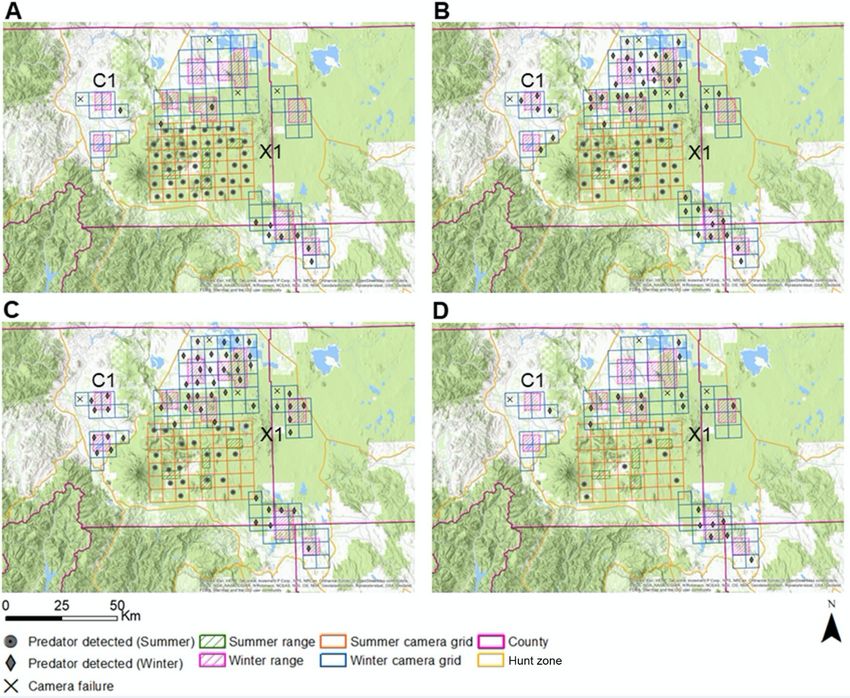
16b) Effect of predation on summer and winter ranges: We also used cameras to
determine the detection and relative abundance of predators at the landscape scale
(deer summer and winter ranges). Cameras were active for various lengths of time
based on field logistics around retrieval, but we aimed to obtain data for 3 continuous
months (90 days) of monitoring for each camera station.
Summer ranges: Between May-June and September 2019, we deployed a total of 48
cameras across a 1,728 km2 area covering all identified summer ranges and the
surrounding landscape. One camera each was placed into a 6 x 6 km (36 km2) grid cell.
The size of the grid cells was based on approximate home range estimates for female
black bears (e.g., Grenfell & Brody 1986, Koehler & Pierce 2003) and were intended to
ensure independence among camera locations. To maximize predator detection, we
generated the centroid of each cell and a circle with 1 km radius that was centered on
the cell centroid. We used high resolution aerial imagery overlaid with terrain in Google
Earth 3D to focus on topographic features within the circle’s radius that could encourage
or funnel predator movement. We selected 3 possible locations for camera station
placement within the circle and entered their coordinates in a hand-held GPS. We
visited one location for camera placement and withheld the other 2 locations as back-
ups in the event ground conditions were unfavorable (i.e., location was in fresh logging
cutblock). We carried out a search within 100 m radius for landscape features that
promoted predator movement and placed a camera at the location that likely maximized
predator detections (e.g., old roads, funnel areas, or game trails).
Winter ranges: Between November 2019 and April 2020, we deployed a total of 84
cameras across a 3,024 km2 area covering all identified winter ranges and a broader
area around these. To enable comparison with summer range data, grid cell size was
the same for summer and winter ranges and camera deployment procedures were
comparable to those described for summer above. Some habitats on winter ranges
were more open than on summer ranges, therefore we could not always rely on
standing trees to affix the cameras and used metal stakes instead.
MOUNTAIN LION CAPTURES & MONITORING
Mountain lion research was approved through a Memorandum of Understanding
between the CDFW and the UCSC. All mountain lion capture and handling procedures
were approved by veterinarians with the Wildlife Investigations Laboratory of the CDFW,
the UCSC Institutional Animal Care and Use Committee (protocols Wilmc1509 &
Wilmc1811), a CDFW Scientific Collection Permit (SC-11968) and adhered to
guidelines established by the American Society of Mammologists (Sikes et al. 2016). All
mountain lion captures were led by a CDFW & UCSC approved capture supervisor.
We deployed baits and monitored these with satellite transmitters and camera traps. We
only set and activated a baited cage trap with a deer carcass if a mountain lion had
visited the bait. To alert us of a mountain lion entering the trap, we attached a trap
monitor (TT4, Vectronic Aerospace, Germany) to the cage. Using a trap monitor allowed
us to reduce the number of times we had to physically check the traps and also to
17minimize the time captured mountain lions spent in the trap prior to processing. The
capture team waited in the vicinity of the trap so that they could respond rapidly in case
of a trap trigger. We darted mountain lions caught in traps using a less powerful Pneu-
Dart compression pistol.
We anesthetized captured mountain lions using Telazol (tiletamine and zolazepam) as
outlined by the CDFW Departmental Policy on the Use of Pharmaceuticals in Wildlife.
We used Telazol at a concentration of 100 mg/ml and administered initial dosages of 2
ml for females and 3 ml for males. We applied Midazolam at a concentration of 5 mg/ml
as needed for improved muscle relaxation. Throughout the handling procedures, we
monitored vital signs including body temperature and respiration rates. We determined
sex of all captured mountain lions and then weighed, measured, and fitted each animal
with an individually numbered ear tag ID. Measurements included curvilinear nose-to-
rump length, tail length, chest girth, head and neck circumferences, foot pad widths, and
several metrics for legs and teeth. We used measurements of gum-line recession to
determine the approximate age of captured mountain lions (Laundré et al. 2000).
Finally, we fitted each mountain lion with a satellite enabled GPS collar (Vertex Plus,
Vectronic Aerospace, Germany) that also collected accelerometer data. Collars could
be remotely re-programmed using satlink and UHF technology and were accessorized
with automatic and on-demand drop-offs to facilitate recovery of the store-on-board
accelerometer and activity data at the end of the collar’s lifetime.
Note that all capture data was provided to CDFW and included in a recent meta-analysis
aimed at determining optimal capture and immobilization procedures for mountain lions in
California (Basto et al. unpublished manuscript).
We programmed GPS collars to acquire locations every 2 h throughout the regular
monitoring period and every 5 minutes during intensive monitoring periods for kill rate
estimation (see mountain lion diet & kill rates below). We accessed location data
through the Vectronic GPS Plus X interface via a UCSC secure server after the collars
had uploaded acquired location data via the satellite.
Note that mountain lion GPS location data from our study animals has been made available
to CDFW and were used in a state-wide analysis to estimate the amount of suitable habitat
for mountain lions across California (Dellinger et al. 2020).
Collars were fit with motion-activated mortality sensors. If a collar was motionless for >
12 h, we were alerted via email to the possibility that the mountain lion had died. We
conducted field investigations immediately after receiving notification of potential
mortality events and used data collected in the field to determine cause of mortality.
This included evidence found directly on the body of the dead mountain lion (e.g.,
entrance wounds from canines or bullets, claw marks) and at the mortality site (e.g.,
tracks, drag marks, blood spatter, vegetation disturbance).
18Note that all mountain lion monitoring data and cause of mortality information has been
provided to the CDFW to be included in a meta-analysis aimed at determining cause-specific
survival estimates for mountain lions in California (Benson, Dellinger et al. unpublished
manuscript).
MOUNTAIN LION POPULATION DENSITY
We estimated the population density of mountain lions based on home range overlap
(Rinehart et al. 2014). We estimated mountain lion densities across a 714 km2 focal
area where we believed we had captured and collared the majority of resident
individuals occupying the area at the time and identified any uncollared mountain lions
based on their tracks. The extensive network of public and logging roads and relatively
mild winter conditions facilitated good coverage of the area in 4×4 vehicles to search for
fresh tracks. Driving was supplemented by hiking in certain areas to maximize our
search effort. Although we were only able to reliably ascertain individual mountain lion
presence from tracks when snow was present on the ground, for comparative purposes
we estimated densities within the focal area both for winter (Nov. 15, 2018 to Feb. 14,
2019) and summer (Jun. 1 to Aug. 31, 2018). Home ranges of mountain lions were
estimated using the kernel plug-in bandwidth method based on GPS locations acquired
at 2 h fix rates during the 3-months periods outlined above (Gitzen et al. 2006).
MOUNTAIN LION DIET & KILL RATES
To determine diet composition of mountain lions, we investigated location clusters
identified by an algorithm initially developed by Knopff et al. (2009) and adapted by the
Santa Cruz Mountain Lion Project (Wilmers et al. 2013) to locate potential kill sites.
Cluster identification was automated and relied on 2 h fix rates of mountain lion collars,
where ≥ 2 fixes were spatio-temporally constrained to occur within 100 m of each other
within a 6 day timeframe (Wilmers et al. 2013). In the field, we carefully approached the
area associated with a location cluster to locate potential prey remains and documented
any evidence that helped us to determine whether it had been killed by a collared
mountain lion or whether the animal had been scavenging. Evidence used to ascertain
that a mountain lion had killed the prey included puncture wounds, bite and claw marks,
broken vegetation, drag marks, animal tracks, and blood spatter. We identified prey
species by their skeletal remains and external characteristics such as hair and feathers
using a field guide (Elbroch & McFarland 2019). For mammals, we also attempted to
identify the sex and age classes of the prey species. Finally, we collected a tooth at
sites where we found remains of deer jaws for exact age determination using cement-
annuli methods (Matson’s Laboratory LLC, Missoula, MT, USA).
To obtain more precise estimates of mountain lion kill rates, we conducted intensive kill
rate monitoring sessions of focal individuals. Kill rate monitoring sessions lasted for 28
days during which time we investigated all clusters where a mountain lion had remained
for ≥ 2 hours. This followed results showing that estimates solely based on
19investigations of longer clusters may bias kill rate estimates of mountain lions (Elbroch
et al. 2018). We estimated kill rates both as the number of ungulates killed per week as
well as ungulate biomass killed per day. To convert estimates based on the number of
ungulates killed per week into biomass we used live weight estimates from different
sources. For deer and elk of all age and sex classes we used data from Oregon (Clark
et al. 2014), except for adult female deer for which we used Siskiyou-specific mean
weight from live capture records for the project. Additional sources were used to obtain
weights of pronghorn (Silva & Downing 1995), feral horse (Knopff et al. 2010), and
cattle (UC 2004).
EFFECT OF SCAVENGERS ON MOUNTAIN LION KILL RATES
To quantify the potential impact of scavengers on mountain lion kill rates, we placed
motion-activated video cameras (XR6, Reconyx, USA) at a subset of kills we
discovered. We only placed video cameras at fresh kills to ensure we could confidently
determine the timing of arrival of scavengers (Allen et al. 2015, 2016). To ensure we
identified kill sites as quickly as possible, we visually identified potential candidate
locations for camera deployment at kills by mapping mountain lion GPS locations in
Google Earth as soon as they became available. We programmed cameras to record 30
s videos when triggered with a 5 s refractory period. Cameras remained active for at
least 3 weeks or until batteries ran out. To limit the ability of scavengers to drag the
carcass out of the field of view of our cameras, we anchored carcasses using rope. We
tagged all videos using software BORIS (Friard & Gamba 2016). To reduce observer
variability, all videos were tagged by the same individual. Variables recorded included
the species triggering the camera, whether the individual(s) fed on the carcass, as well
as the duration of feeding bouts. For mountain lions we developed a more complex
ethogram that included behavioral states that were not restricted to feeding (e.g.,
resting, caching). We used the camera data to compare feeding times of mountain lions
at carcasses with vs. without bear visitation.
RESULTS
SEASONAL DEER RANGES & MOVEMENTS
Based on available deer GPS location data in 2017, we identified 9 potential winter
ranges. We also delineated 4 summer fawning ranges. Both winter and summer ranges
are shown on Fig. 2.
20Fig 2. Summer (green, n = 4) and winter (white & yellow, n = 9) ranges of deer delineated as
part of the Siskiyou deer-puma study in northern California between 2015-2020. One of the
winter ranges (yellow rectangle) is a high elevation area that received little use based on deer
pellet transect data and was therefore not included in our vegetation surveys. Seasonal ranges
are overlaid with Level IV ecoregions (Environmental Protection Agency 2012) present in
California.
We used 88 animal years from 78 unique adult female deer (i.e., we had two animal
years’ worth of data for 10 individuals) for our movement classification analysis. Of the
88 animal years, 4 were classified as residents, 67 as migrants, and we were unable to
confidently classify the remaining 17 animal years to a specific movement strategy.
Deer migrated an average of 53.5 km (n = 67, range = 12.7-83.9 km) between seasonal
ranges. Seasonal migration strategies were complex and will require further
investigation.
21Approximately 10% of migratory animal years crossed HWY 97 (i.e., 7 out of 67,
representing n = 60 unique individuals). None of the 7 individuals we had multiple
animal-years classifications for crossed HWY 97, thus the effective percentage on an
individual basis would be 7/60 or approximately 12%. Some deer crossed HWY 89, but
none of these deer were classified as migratory. Seasonal migration corridors are
highlighted in Fig. 3.
Fig. 3. Seasonal migration corridors between summer and winter ranges delineated as part of
the Siskiyou deer-puma study in northern California between 2015-2020. Corridors based on
GPS location data of 60 adult female deer.
FAWN CAPTURES
Between June 2016 and June 2019, we captured and collared a total of 145 fawns
(67F/78M). Only 4 fawns (2F/2M) were captured during our pilot study in 2016. Annual
sample sizes of collared fawns in subsequent years were 38 (14F/24M) in 2017, 51
(27F/24M) in 2018, and 52 (24F/28M) in 2019. The earliest fawn capture date was June
4, and the latest capture date was July 4. Only 3 fawns overall were captured in July.
Both mean (18 June, 19 June, 19 June) and median (21 June, 20 June, 19 June)
capture dates were similar across all 3 years with comparable capture efforts. Weights
of fawns at capture averaged 4.71 kg (±1.49 SD) and ranged from 2.30 kg to 8.90 kg.
22You can also read