The Consequences of the Brexit Vote for UK Inflation and Living Standards: First Evidence
←
→
Page content transcription
If your browser does not render page correctly, please read the page content below
The Consequences of the Brexit Vote for
        UK Inflation and Living Standards: First Evidence
       Holger Breinlich          Elsa Leromain             Dennis Novy            Thomas Sampson∗

                                             January 2019

                                                 Abstract

        We analyze the impact of the Brexit referendum in June 2016 on UK inflation and
        living standards. We propose a theoretical framework in which households are ex-
        posed to imported goods directly through the consumption of foreign final goods
        and indirectly through the use of foreign intermediates in domestic production. We
        generate empirical measures of the direct and indirect exposure to imported goods
        based on UK input-output tables. The pound depreciated by around 10% immediately
        following the referendum and we show that product groups with larger direct and
        indirect import shares experienced higher inflation after the vote. Our results suggest
        that the referendum increased aggregate UK inflation by 1.7 percentage points within
        one year. Exploiting differences in expenditure patterns across household types we
        find that the increase in inflation is evenly shared across the income distribution, but
        not across regions. London is the least affected region, while Scotland, Wales and
        Northern Ireland are hardest hit. We conclude that voting to leave the EU has already
        raised the cost of living for UK households.

        Keywords: B REXIT, I NFLATION , T RADE , I MPORTS , I NTERMEDIATES , E XCHANGE R ATE
        JEL Classification: E31, F15, F31

   ∗
    This technical report details the analysis described in Centre for Economic Performance (CEP) Brexit
Analysis No. 11 “The Brexit Vote, Inflation and UK Living Standards”. The research is supported by the UK’s
Economic and Social Research Council through the UK in a Changing Europe initiative under Brexit Priority
Grant ES/R001804/1. All four authors are affiliated with the CEP at the London School of Economics. Breinlich:
University of Nottingham, Leromain: London School of Economics, Novy: University of Warwick, Sampson:
London School of Economics. Email addresses: holger.breinlich@nottingham.ac.uk, e.leromain@lse.ac.uk,
d.novy@warwick.ac.uk, t.a.sampson@lse.ac.uk.
1 Introduction
The result of the Brexit referendum held on 23 June 2016 took many observers by sur-
prise. The British electorate voted to leave the European Union with a majority of 51.9%.
As soon as the eventual vote outcome became clear during the referendum night, the
pound depreciated sharply against the US dollar and the euro. This decline in the ex-
change rate persisted in the subsequent months, with sterling still around 10% below
its pre-referendum value by November 2017. The decline in the value of the pound is
consistent with the referendum outcome causing market participants to downgrade their
expectations about the future performance of the UK economy. Both increased uncertainty
and the likelihood that the UK would in future become less open to trade, investment and
immigration with the EU probably contributed to this downgrade in expectations.
Standard economic theory predicts that a strong and sustained depreciation of a country’s
exchange rate should lead to an increase inflation by raising the cost of imports. In fact,
CPI inflation in the United Kingdom rose from 0.5% in June 2016 to to 2.6% in June 2017
and 3.0% in September 2017. To what extent can we attribute this rise in inflation to the
Brexit vote and subsequent exchange rate depreciation, compared to other factors such as
changes in oil prices and inflationary pressures resulting from faster growth in the Euro
area and the US?
In this technical report we estimate the impact of the Brexit vote on CPI inflation in the
UK, focusing primarily on how the exchange rate shock following the referendum affected
inflation. We treat the referendum outcome, and the resulting exchange rate depreciation,
as an unanticipated shock to the UK economy and study their consequences. After account-
ing for other determinants of inflation, we find that products with a larger import share in
consumer expenditure experienced higher inflation following the referendum. This shows
that the exchange rate depreciation caused by the Brexit vote has put upwards pressure on
inflation. We find evidence that higher import prices for both final goods and intermediate
inputs used by UK producers have contributed to the rise in inflation.
Section 2 of the report lays out a theoretical framework to motivate our estimation
approach. Section 3 describes the data we use and how we construct our main variables.
Section 4 introduces our estimation specification and Section 5 presents the results.
Finally, Section 6 discusses the implications of our findings for aggregate inflation and for
differences in inflation rates across household types, before Section 7 concludes.
22 Theoretical framework
We are interested in how UK consumer prices changed after the referendum shock led to
the depreciation of sterling. Building on Berlingieri, Breinlich and Dhingra (2017), we
sketch a framework that will provide the basis of our empirical strategy.
The representative household in the domestic economy derives utility from the consump-
tion of a basket of G goods.1 The consumption of good g, Cg , is a composite of an imported
good Mg and a domestic good Dg such that
γ 1−γg
Cg = M g g D g ,
with γg being the share in the total consumption of g that the household spends on the
imported good. We can express the logarithmic change in the consumer price index for
good g as
Pg,t PgM,t PgD,t
ln = γg ln + (1 − γg ) ln , (1)
Pg,t−1 PgM,t−1 PgD,t−1
where Pg,t is the price index for the composite good g in period t, and PgM,t and PgD,t are
the prices of the imported and domestic goods. The first term on the right-hand side of
equation (1) indicates that a change in the price PgM,t of the imported good feeds into
the price index Pg,t directly through household expenditure. In addition, a change in the
price of the imported good also feeds into the price index indirectly to the extent that
the imported good is used as an input in the production of the domestic good and thus
affects PgD,t . The magnitude of the direct effect crucially depends on the value of γg . The
magnitude of the indirect effect depends on how much the price of the domestic good is
affected by changes in intermediate input prices.
We assume that the production of the domestic good g requires a primary factor (e.g.,
labour), and a bundle of domestic and imported intermediate inputs. More specifically, the
production function of the representative domestic firm in sector g is
αg
yg = φg l1−αg iDg 1−εg iM g εg ,
where φg is total factor productivity (TFP), l is the primary factor, iDg is the domestic
intermediate input and iM g is the imported intermediate input, αg denotes the share
of total intermediate consumption in gross output of sector g, and εg is the share of
imported intermediates in total intermediate consumption. With a perfect pass-through
1
We use “goods” to refer to any product consumers purchase. In the empirical implementation this will
cover both goods and services.
3from production costs to prices, this technology implies a price ratio for domestic good g of
−1 1−αg 1−εg εg !αg
PgD,t φg,t wt PgID,t PgIM,t
= , (2)
PgD,t−1 φg,t−1 wt−1 PgID,t−1 PgIM,t−1
where wt is the factor price for the primary factor, PgID,t is the price index of the domestic
intermediate input and PgIM,t is the price index of the imported intermediate input. The
exchange rate shock can affect prices through changes in TFP, factor prices and the cost of
intermediate inputs (domestic or imported). Given the difficulty of convincingly identifying
productivity and factor prices effect (to the extent they exist), we focus on intermediate
inputs for now. However, we will allow for general equilibrium effects more broadly in our
empirical results. Without changes in TFP or factor prices, the price ratio for the domestic
good can then be expressed as
1−εg εg !αg
PgD,t PgID,t PgIM,t
= . (3)
PgD,t−1 PgID,t−1 PgIM,t−1
We assume that the domestic input bundle for sector g is produced using the output of all
other sectors in the economy. Hence, its price ratio is given by
G
PjD,t ψjg
PgID,t Y
= , (4)
PgID,t−1 PjD,t−1
j=1
where ψjg is the share of intermediate expenditure on group j by group g in total domestic
intermediate expenditure. Note that the prices on the right-hand side of equation (4)
correspond to the last term of equation (1). Similarly, we assume that the imported
intermediate bundle consists of imported inputs from all other sectors. The ratio of the
imported input price can hence be written as
G
PjM,t µjg
PgIM,t Y
= , (5)
PgIM,t−1 PjM,t−1
j=1
where µjg is the share of intermediate expenditure on group j by group g in total imported
intermediates. The prices on the right-hand side of equation (5) correspond to the first
term on the right-hand side of equation (1).
Combining equations (3) and (4), we can express the ratio of the domestic good price as
ψjg αg (1−εg )
G
PgIM,t αg εg
PgD,t Y PjD,t
= . (6)
PgD,t−1 PjD,t−1 PgIM,t−1
j=1
4Taking the logarithm of equation (6) we obtain
G
PgD,t X PjD,t PgIM,t
ln = αg (1 − εg )ψjg ln + αg εg ln . (7)
PgD,t−1 PjD,t−1 PgIM,t−1
j=1
Note that we have G such equations for the entire economy (one per good). We can
rewrite this system in matrix notation as
−−−→ −−−→ −−−−→
∆PD = ΩD ∆PD + ΩM ∆PIM , (8)
−−→
where ∆P are G × 1 column vectors of logarithmic price changes. ΩD is a G × G matrix
D , equal to α (1 − ε )ψ . Ω
with the element of row g and column i, ωgi g g ig M is a G × G
diagonal matrix with the ith element on the diagonal, ωiiM , equal to αi εi . Solving for the
−−−→
vector of domestic good price changes, ∆PD , we arrive at
−−−→ −−−−→
∆PD = (I − ΩD )−1 ΩM ∆PIM . (9)
where I is the G × G identity matrix. Given the change in imported good prices, we
can infer the change in the price of the imported input goods from equation (5) and
subsequently the change in the price of domestic goods from equation (9).
To study the effect of the exchange rate shock, we assume that the change in imported
goods prices is identical across sectors. We will be more specific about how we measure
the size of the shock below, but for now we simply denote it as β, i.e.,
PgM,t
ln = β ∀g = 1, . . . , G.
PgM,t−1
Hence, the direct effect is βγg in equation (1), while the indirect effect is the product of
−−−−→
1−γg and the change in domestic good prices. From equation (5), it follows that ∆PIM is a
−−−→
G×1 column vector with all elements equal to β. Hence, we have ∆PD = (I − ΩD )−1 ΩM β.
From equation (1), the vector of overall price changes is then
−−→
∆P = Ωγ β + Ω1−γ (I − ΩD )−1 ΩM β, (10)
where Ωγ and Ω1−γ are G × G diagonal matrices with the ith elements on the diagonals
equal to γi and 1 − γi , respectively.
This system of equations will form the basis of our estimation. For what follows, it is
instructive to look at the price change in one particular sector g (corresponding to equation
g in the system)
5G G
!
Pg,t X X
ln = γg β + (1 − γg ) ωgi β = γg + (1 − γg ) ωgi β, (11)
Pg,t−1
i=1 i=1
where ωgi is the element of row g and column i of the G × G matrix (I − ΩD )−1 ΩM .
Equation (11) tells us that the referendum shock β has a direct effect on prices of good g
that depends on the import share (through γg ), and an indirect effect that depends on the
input-output linkages of intermediates used in the production of g (through the remaining
terms). As indicated by the parentheses on the right-hand side of equation(11), we can
also compute a summary measure of these two effects by simply adding up the direct and
indirect effects and multiplying them by the size of the shock, β. Correspondingly, in our
empirical analysis we will present results for the summary measure as well as separately
for the direct and indirect effects.
3 Data
3.1 Inflation
To measure UK inflation in a way consistent with equation (1), we use the logarithmic
price ratio (i.e., the growth rate in prices) for a given product g. We use price indices
provided by the Office for National Statistics (ONS) for 84 products collected at monthly
frequency. A product is defined as one COICOP (Classification of Individual Consumption
according to Purpose) class.2 The price index for each class is defined the average price of
goods and services within that class bought for the purpose of consumption by households
in the UK and foreign visitors to the UK.3
Our estimates use both annual and quarterly measures of inflation. Since the referendum
occurred in late June we define annual inflation for year t as the logarithmic ratio of the
class price index in June of year t over the price index in June of year t − 1. Our annual
estimates use inflation data for June 2015, June 2016 and June 2017. Quarterly inflation
is computed as the ratio of the class price index in the last month of the quarter over the
class price index in the last month of the previous quarter. Our quarterly estimates use
data from the first quarter of 2015 to the third quarter of 2017.
3.2 Measuring import exposure
To test to what extent inflation following the referendum is due to the exchange rate
depreciation, we need to build a product-specific measure of import exposure, denoted
ImportShare. Based on equation (11), we compute this measure as the sum of two
2
We choose to use price data at the COICOP class level because it approximately matches the level of
aggregation used in the UK input-output tables.
3
See the Consumer Price Indices Technical Manual published by the ONS for more details.
6terms: a direct import exposure measure, DirectImportShare, and an indirect exposure
measure, IndirectImportShare. From equation (11) the direct exposure is simply given
by consumer expenditure on imported goods, γg . In the UK input-output tables we observe
for each sector the value of household expenditure on both domestic and imported goods,
and we calculate γg as the expenditure on imported goods g over total household expen-
diture (domestic and imported) on g. We base our calculations on the UK input-output
analytical tables for the year 2013, which is the most recent version available from the ONS.
Indirect import exposure is the product of (1 − γg ) and the change in the price of domestic
good g. From equations (10) and (11), the latter is determined by the elements of the ΩD
and ΩM matrices which can be calculated using UK input-output tables. We compute αg
as total intermediate consumption (domestic and imported) over total output of sector g.
Similarly, we compute εg as total imported intermediate expenditure over total intermedi-
ate consumption in sector g. Finally, ψjg is the intermediate expenditure on domestic good
j for the production of good g over total intermediate expenditure for the production of
good g.
The sectors in the UK input-output tables are defined according to the Statistical Classifica-
tion of Products by Activity (CPA). To map our import share measure to the classification
used for inflation, we need to convert from CPA sectors to COICOP classes. We use a
CPA-COICOP concordance table provided by the ONS that maps to 115 COICOP classes.
We then aggregate across some classes to obtain import share measures for the COICOP
classes used in the Harmonised Index of Consumer Prices (HICP).4 The ONS publishes
price data for 85 COICOP classes, but we drop Second-hand cars because we are unable to
calculate the indirect import share for Second-hand cars.
3.3 Measuring the exchange rate depreciation
We now return to the measurement of the change in import prices, ln (PgM,t /PgM,t−1 ). In
our baseline estimation, we will simply regress changes in annual or quarterly inflation
on our ImportShare measure, or separately on its two components, DirectImportShare
and IndirectImportShare. The change in import prices is then implicitly given by the
regression coefficient on these measures (i.e., β in equation (11)).
As an alternative, we use actual changes in the exchange rate faced by UK importers,
∆XRt , to proxy for changes in price indices of imported goods. In particular, we assume
PgM,t
ln = βe ∆XRt ∀g = 1, . . . , G.
PgM,t−1
4
We compute arithmetic means of our measures whenever aggregating across classes.
7where βe measures the pass-through from exchange rate changes to import prices, and the
computation of ∆XRt is described below. Given this assumption we compute an exchange
rate measure for each good g in each period t that is the sum of two components: a direct
exchange rate measure and an indirect exchange rate measure. Note that these are simply
DirectImportShare and IndirectImportShare multiplied by ∆XRt . Analogous to our
import share measure, an increase in the exchange rate measure captures an increase in
the relative price of imported goods.
The exchange rate change faced by UK importers, ∆XRt , is a trade-weighted mean of
exchange rate changes given by
X XRc,t
∆XRt = wc × ln ,
c
XRc,t−1
where the import weight wc is the share of partner c in total UK imports, and XRc,t is
denominated as sterling per unit of foreign currency of country c at time t such that an
increase represents a depreciation of sterling. The import weights are calculated from UN
Comtrade using UK imports across all goods from 176 partner countries for the year 2013.5
The exchange rate data are taken from the International Financial Statistics database
provided by the International Monetary Fund (IMF), and the missing data points are
filled in using the online currency converter service Oanda. Analogous to the definition of
annual inflation, the annual exchange rate change is taken as the logarithmic ratio of the
exchange rate in June of year t over the exchange rate in June of year t − 1. The quarterly
change is the logarithmic ratio of the average exchange rate during the quarter over the
average during the previous quarter.
3.4 Other variables
To disentangle the effect of the referendum from other factors that may influence inflation-
ary trends in the UK, we employ two additional variables. The first is a measure of inflation
in the Euro area. We use the price index for each COICOP class from the Harmonized
Index of Consumer Prices (HCIP) provided by Eurostat. This aggregate is computed from
the HICP of the nineteen Euro area countries. For the UK, the HICP is the same as the CPI
produced by the ONS.
The second measure aims at capturing the effect of oil price changes on input prices
through direct or indirect imported oil use in the UK. To capture the impact of changes
in imported crude oil on UK consumer price indices, we follow a similar methodology as
for the import share measure. However, it turns out the oil measure only has an indirect
component because households do not directly consume or import crude oil (i.e., γoil = 0).
5
The year was chosen to be consistent with the year of the UK Input-Output tables.
8The indirect component is fully determined by changes in domestic prices due to changes
in the imported crude oil price. We assume
PgM,t
ln Poil,t if g ∈ {Oil},
Poil,t−1
ln =
PgM,t−1 0 otherwise.
−−−−→
To determine ∆PIM we need µoil,g , which is the intermediate expenditure on imported
crude oil over total expenditure on imported intermediates for good g. This can be retrieved
from the imported use table provided in the UK input-output tables. Once we determine
−−−−→
∆PIM , we compute the changes in domestic prices due to changes in imported crude oil,
−−−→
∆PD , using equation (9). To proxy changes in crude oil prices we use the APSP (Average
Petroleum Spot Price) crude oil index provided by the IMF Commodity Price database. It
is an average index of prices of Brent crude, Dubai and West Texas Intermediate crude.
Descriptive statistics for all our variables are shown in Table 1.
4 Empirical specification
We implement a difference-in-differences approach to quantify to what extent the rise
of inflation following the referendum is due to an increasing cost of imports. For that
purpose we analyze the UK inflation trend before and after the referendum and distinguish
products by degree of import exposure.
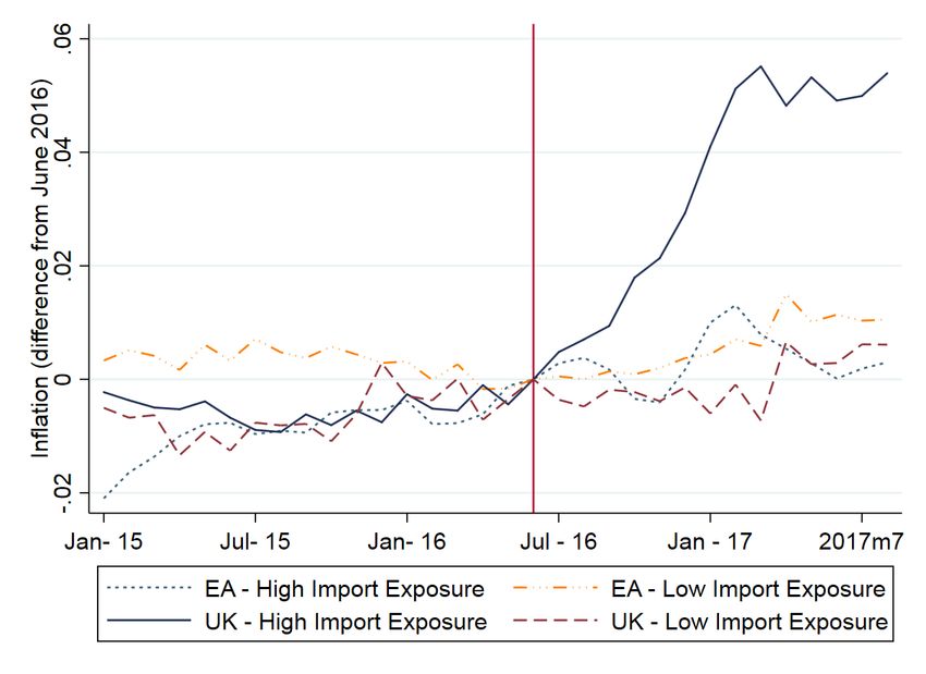
Figure 1: Inflation rates by import exposure measure
As motivation, Figure 1 displays both UK and Euro area (EA) inflation rates with respect to
9the same month in the previous year. The solid line is the UK average inflation rate for
products with high import exposure, while the dark dashed line is the average inflation rate
for products with low import exposure. The dotted line is the Euro area average inflation
rate for products with high import exposure, while the grey dashed-dotted line is the Euro
area average inflation rate for products with low import exposure. For each of the four
groups, the inflation rate is expressed as the difference from the average group inflation
rate in June 2016. High import exposure products are those with an import exposure
measure above the median; other products are counted as low import exposure. The
trend in inflation for these groups of products is similar before the referendum but clearly
different afterwards. Inflation increases drastically after the referendum for products with
high import exposure in the UK, consistent with the notion that this diverging trend may
be due to increasing import costs.
More formally, we estimate the following equation for 84 COICOP classes g:
Inf lationgt = β(P ost × ImportShare)gt + Xgt + δt + δg + εgt . (12)
The dependent variable Inf lation is the inflation rate for a given COICOP class in period
t. P ost is a dummy variable that takes the value 1 for all periods after the referendum.
ImportShare is the import exposure measure that captures both the direct and indirect
increases in import costs. Xgt are additional factors that are likely to influence inflationary
trends in the UK, namely the measure of the impact of oil price changes on domestic good
price g in period t, Oil, and the measure of euro area inflation for a given product g in
period t, EuroAreaInf lation. Period fixed effects and product fixed effects are denoted
by δt and δg . The coefficient of interest is β. It captures the effect of the referendum that
is channelled through rising import costs. We expect β to be positive. Alternatively, we
estimate equation (12) interacting P ost with the ExchangeRate measure.
5 Estimation results
Tables 2 and 3 report the results of estimating equation (12) at annual frequency. Table
2 displays the total effect of the referendum as captured by the interaction between the
P ost dummy and the overall ImportShare measure. Table 3 distinguishes between the
direct effect (captured by the interaction of the P ost dummy and the DirectImportShare
measure) and the indirect effect (captured by the interaction of the P ost dummy and the
IndirectImportShare measure). In both tables, columns (2) to (3) introduce controls one
at a time. Product fixed effects as well as annual dummies for 2015 and 2017 are included
in all regressions.6
6
To avoid possible confusion, recall that the annual data for year t covers the period between June in year
t − 1 and June in year t. Thus, the 2017 fixed effect covers the post-referendum period after June 2016.
10Our preferred specification is presented in column (3) where we control for both changes in
oil prices and the inflationary trend in the euro area. In column (4) we use the alternative
dependent variable Inf lation Dif f erence, which is the difference between UK and Euro
area inflation for a given product in a specific year. In column (5) we decompose the timing
in the referendum effect by interacting the import share measure with individual year
dummies rather than the P ost dummy (the omitted reference period is 2015). Overall,
the estimated β coefficients are positive, statistically significant and rather stable across
the various specifications. Products with higher import exposure experienced a greater
increase in inflation following the referendum.
Recall that interpreted through the lens of our model, the coefficient on the import share
regressor captures the change in import prices. According to our preferred coefficient
estimate of 0.0709 (Table 2, column 3) this means that import prices increased by around
7% post-referendum. Given that the trade-weighted exchange rate depreciated by around
10%, the implied-pass through rate seems plausible and consistent with the wider literature
on exchange rate pass-through. Moreover, for our preferred specification we cannot reject
the hypothesis that the coefficients on our direct and indirect import share measures are
the same (Table 3, column 3), as consistent with our theoretical framework.
Tables 4 and 5 report the results of estimating equation (12) at quarterly frequency.
Columns (1) to (4) of Table 4 are similar to columns (1) to (4) of Table 2. In column
(5) we introduce P eriod × division fixed effects. A division refers to a 2-digit COICOP
code, and there are 12 COICOP divisions in total. In column (6) we estimate the direct
and indirect effects separately. The quarterly results are broadly consistent with annual
estimates: the β coefficients are positive, statistically significant and rather stable across
the various specifications. In particular, products with higher import exposure experienced
a greater increase in inflation following the referendum.
Table 5 decomposes the effect by quarter for the overall measure in column (1), and for
the direct and indirect measures in column (2). The interaction of the quarter dummies
and the import share measures is always insignificant prior to the referendum and then is
positive and significant in all quarters after the referendum except for the second quarter
of 2017, at least for the total and direct import share measures.
Table 6 reports the results of estimating the baseline specification at the quarterly frequency
using exchange rate changes to capture import price changes. We add lags to allow for
delayed pass-through from the exchange rate to domestic prices. In column (1) we use
our composite exchange rate regressor whereas in column (2), we decompose the total
11effect into direct and indirect effects as before. Column (1) indicates that exchange rate
depreciations increase domestic inflation with a lag of one to two quarters, with the
strongest effects visible after two quarters and the three-quarter lag not being statistically
different from zero. This timing is broadly consistent with column (1) of Table 5 where
we found significantly positive effects from the third quarter of 2016 through to the first
quarter of 2017. When we split up the total exchange rate effect into its direct and indirect
components (column 2), we find that the direct effect is similar to the aggregate effect
from column (1). The indirect effects are very imprecisely measured, however, with all
lags being statistically insignificant.
6 Aggregate inflation
Using our annual estimates along with prices and CPI weights for COICOP classes, we can
compute an aggregate counterfactual rate of inflation and compare it with the actual rate
of inflation to capture the overall referendum effect. We define the counterfactual rate of
inflation as P84 !
C
g=1 w2016,g P2017,g
Inf lationRateC
2017 = P84 −1 ∗ 100,
g=1 w2017,g P2016,g
where w2017,g is the weight of product g in the aggregate index in 2017, w2016,g is the
weight of product g in the aggregate index in 2016, P2016,g is the price for product g in 2016
C
and P2017,g is the counterfactual price for product g in 2017. Under the assumption that the
referendum affects prices only through increasing import costs, we compute the counter-
C
factual price for product g in 2017 as P2017,g = P2017,g /eBg with Bg = β̂ ∗ ImportShareg .
However, the referendum might have affected inflation through other channels. For exam-
ple, if the vote led to an increase in wages or other domestic production costs, then we
would expect prices to rise in all sectors of the economy. Alternatively, if producers expect
Brexit to lead to slower future growth they may choose smaller price increases leading
to lower inflation. To account for such potential general equilibrium effects, we compute
GE
C
the counterfactual price as P2017,g = P2017,g /eBg with BgGE = β̂ ∗ ImportShareg + δ̂ 2017 ,
where we interpret the 2017 period dummy as absorbing these other effects.7
The referendum effects are expressed as percentage point increases in inflation over the
period from June 2016 to June 2017. In all specifications in Table 2 the general equilibrium
adjustment as captured by the 2017 dummy is negative. Our estimate (excluding the
general equilibrium adjustment) would then be an upper bound of the referendum effect.
More specifically, based on our estimate for β in column (3) of Table 2, we find that the
referendum increased inflation by 3.17 percentage points in the year after the referendum
(excluding the general equilibrium adjustment). Accounting for general equilibrium effects,
7
When computing the aggregate inflation effect we assign Second-hand cars an import share of zero.
12we find that the referendum increased inflation by 1.71 percentage points. We regard this
overall referendum shock effect as a conservative estimate of the impact on aggregate
inflation since we choose to attribute the entire negative general equilibrium effect to the
Brexit vote.
It is useful to compare this baseline estimate of the referendum effect with the effect
implied by the estimates in column (1) of Table 6, which uses quarterly data and includes
exchange rate movements both before and after the referendum to capture import price
changes. We apply the approach described above to calculate counterfactual inflation
rates for each quarter from the third quarter of 2016 to the second quarter of 2017. We
then combine these quarterly impacts to obtain an estimate of the overall referendum
effect between June 2016 and June 2017. When calculating the counterfactual inflation
rates we use the estimated effect of the first and second exchange rate lags only, as the
other exchange rate variables are all insignificant. We also do not include any general
equilibrium adjustment. Our estimates suggest there may have been a positive general
equilibrium effect in the second quarter of 2017, but to obtain a conservative estimate of
the impact on aggregate inflation we do not account for this effect.
The import weighted quarterly average exchange rate depreciated by 2.0% in the second
quarter of 2016 and 7.9% in the third quarter of 2016. Attributing both these changes
to the referendum implies the referendum increased inflation by 2.28 percentage points
in the year after the vote. Alternatively, if we take a more conservative approach and
only attribute the change in the third quarter to the impact of the referendum, we obtain
an increase in inflation of 1.57 percentage points. Both these estimates are similar in
magnitude to our baseline result.
6.1 Distributional consequences
In addition, to explore the distributional consequences of the referendum shock due to
variation in expenditure patterns across households, we compute aggregate indices specific
to certain types of households. The ONS provides expenditure for each of our 84 products
by disposable income decile, age and region. Using ONS expenditures from the Family
Spending tables for the financial year ending 2016 we compute household-specific weights
and use the corresponding weights to calculate group-specific aggregate effects.
The results are displayed in Table 7. The increases in inflation rates by household type are
computed using the estimates from our preferred specification (Table 2, column 3) includ-
ing general equilibrium effects. Inflation varies little across income deciles, implying that
the costs from the referendum shock are evenly shared throughout the income distribution.
We conclude that the referendum increased inflation by approximately the same amount
13for poor, middle income and rich households.
By contrast, there are significant differences across age groups and regions. Increases in
inflation rates are substantially lower for households under 30 and households living in
London because these groups spend relatively more on rent than the average household
and rent has a very low import share. In general the north of England is harder hit than the
south. Scotland, Wales, and Northern Ireland are the worst affected areas. Our estimates
imply inflation in Northern Ireland increased by 0.47 percentage points more than the UK
average because of the Brexit vote. This is because households in Northern Ireland spend
relatively more on food and drink, clothing and fuel which are high import share product
groups and relatively less on rent and sewerage which have low import shares.
7 Conclusion
We present a theoretical model in which households consume both domestic and imported
foreign goods. This directly exposes households to inflation stemming from price rises in
imported goods. In addition, households are indirectly exposed to price rises in imported
intermediate goods since those are used as inputs in the production of domestic consump-
tion goods. The model thus delivers a relationship between inflation and the exposure to
imported goods.
On the empirical side, we employ UK input-output tables to construct measures of import
exposure at the product level. We then relate those measures to the UK inflation experience
before and after the June 2016 Brexit referendum, also controlling for the effect of oil
price changes and inflation in the Euro area. We observe a positive relationship across
products between import exposure and price increases following the referendum. Our
preferred point estimate is that the referendum shock led to an increase in aggregate UK
inflation by 1.7 percentage points in the year following the referendum.
We also consider how household expenditure shares differ by income, age and regions,
and we then calculate how the referendum shock affects these groups differentially. We
find that the inflation increase is shared evenly throughout the income distribution but not
across regions. London is the least affected while Scotland, Wales and Northern Ireland
experience the strongest increases in inflation. Young people are less affected because they
spend a larger share of their income on items that are hardly affected by foreign imports,
in particular rents.
14References
Berlingieri, G., H. Breinlich and S. Dhingra (2017), “The Impact of Trade Agreements on
Consumer Welfare - Evidence from the EU Common External Trade Policy,” forthcoming,
Journal of the European Economic Association.
15Table 1: Descriptive statistics
VARIABLES Mean Median Standard deviation Min Max
Inflation 0.006 0.012 0.044 -0.296 0.134
Import share 0.507 0.564 0.318 0.010 0.999
Direct import share 0.386 0.400 0.352 0 0.999
Indirect import share 0.121 0.108 0.089 0.001 0.444
Exchange rate measure 0.017 0.015 0.043 -0.064 0.095
Direct exchange rate 0.013 0.001 0.038 -0.064 0.095
Indirect exchange rate 0.004 0.005 0.0108 -0.028 0.042
Oil -0.006 -0.010 0.023 -0.181 0
Euro area inflation 0.007 0.009 0.032 -0.219 0.256
Notes: The variables Import share, Direct Import share, and Indirect Import share are time-
invariant. The descriptive statistics for these variables are computed on 84 observations. All
other statistics are computed using annual observations (252 observations).
16Table 2: Annual specification: Import share
(1) (2) (3) (4) (5)
VARIABLES Inflation Inflation Inflation Inflation Difference Inflation
Post × Import share 0.0760*** 0.0709*** 0.0709*** 0.0706***
(0.0185) (0.0148) (0.0140) (0.0141)
2016 × Import share -0.00295
(0.0106)
2017 × Import share 0.0694***
(0.0155)
Oil 0.846** 0.672** 0.232 0.673**
(0.393) (0.296) (0.164) (0.297)
Euro area inflation 0.282 0.283
(0.201) (0.200)
2015 dummy -0.00996** -0.00449 -0.00510 -0.00666 -0.00659
17
(0.00394) (0.00410) (0.00399) (0.00499) (0.00637)
2017 dummy -0.0123* -0.0136** -0.0146** -0.0170* -0.0153**
(0.00735) (0.00662) (0.00693) (0.00861) (0.00720)
Observations 252 252 252 252 252
R-squared 0.337 0.459 0.491 0.256 0.491
Number of products 84 84 84 84 84
Product fixed effects YES YES YES YES YES
Notes: The dependent variable in columns (1)-(3) and (5) is the annual UK inflation rate. In column (4)
it is the difference between the UK and Euro area annual inflation rates. Post is a dummy variable for the
post-referendum period. Sample covers 2015-17. We define year t as the period from June of year t − 1 to
June of year t. See the main text for additional details. Constant not reported. OLS estimation. Standard
errors in parentheses clustered by product. *** pTable 3: Annual specification: Direct and indirect import shares
(1) (2) (3) (4) (5)
VARIABLES Inflation Inflation Inflation Inflation Difference Inflation
Post × Direct import share 0.0916*** 0.0760*** 0.0719*** 0.0612***
(0.0209) (0.0147) (0.0126) (0.0126)
Post × Indirect import share 0.310** 0.138** 0.0850* -0.0520
(0.125) (0.0597) (0.0499) (0.0669)
2016 × Direct import share -0.00606
(0.0122)
2017 × Direct import share 0.0673***
(0.0154)
2016 × Indirect import share -0.0479
(0.0572)
2017 × Indirect import share 0.0432
18
(0.0778)
Oil 0.729* 0.651* 0.447* 0.741*
(0.391) (0.328) (0.227) (0.393)
Euro area inflation 0.277 0.264
(0.206) (0.207)
2015 dummy -0.00996** -0.00524 -0.00525 -0.00527 -0.0128
(0.00395) (0.00399) (0.00396) (0.00498) (0.0100)
2017 dummy -0.0466** -0.0231** -0.0166** 0.000453 -0.0182**
(0.0204) (0.00989) (0.00736) (0.00978) (0.00717)
Observations 252 252 252 252 252
R-squared 0.409 0.462 0.491 0.268 0.492
Number of products 84 84 84 84 84
Product fixed effects YES YES YES YES YES
Notes: The dependent variable in columns (1)-(3) and (5) is the annual UK inflation rate. In column (4) it is the
difference between the UK and Euro area annual inflation rates. Post is a dummy variable for the post-referendum
period. Sample covers 2015-17. We define year t as the period from June of year t − 1 to June of year t. See the main
text for additional details. Constant not reported. OLS estimation. Standard errors in parentheses clustered by product.
*** pTable 4: Quarterly specification
(1) (2) (3) (4) (5) (6)
VARIABLES Inflation Inflation Inflation Inflation Difference Inflation Inflation
Post × Import share 0.0199*** 0.0189*** 0.0195*** 0.0205*** 0.0176***
(0.00442) (0.00377) (0.00378) (0.00409) (0.00419)
Post × Direct import share 0.0172***
(0.00407)
Post × Indirect import share 0.0110
(0.0135)
Oil 0.597** 0.438** 0.196* 0.483** 0.487**
(0.274) (0.214) (0.114) (0.219) (0.218)
Euro area inflation 0.395 0.374 0.374
(0.238) (0.242) (0.242)
19
Observations 840 840 840 840 840 840
R-squared 0.036 0.090 0.178 0.033 0.281 0.281
Number of products 84 84 84 84 84 84
Product fixed effects YES YES YES YES YES YES
Period fixed effects YES YES YES YES NO NO
Period × division fixed effect NO NO NO NO YES YES
Notes: The dependent variable in columns (1)-(3) and (5)-(6) is the quarterly UK inflation rate. In column (4) it is the difference
between the UK and Euro area quarterly inflation rates. Post is a dummy variable for the post-referendum period. Sample covers Q1
2015-Q2 2017. See the main text for additional details. Constant not reported. OLS estimation. Standard errors in parentheses
clustered by product. *** pTable 5: Quarterly specification: Decomposition
(1) (2)
VARIABLES Inflation Inflation
2015Q2 × Import share -0.00688
(0.00765)
2015Q3 × Import share 0.00345
(0.00934)
2015Q4 × Import share -0.00425
(0.00880)
2016Q1 × Import share 0.00840
(0.00835)
2016Q2 × Import share -0.00318
(0.00931)
2016Q3 × Import share 0.0188**
(0.00860)
2016Q4 × Import share 0.0236*
(0.0122)
2017Q1 × Import share 0.0454***
(0.0127)
2017Q2 × Import share -0.0114
(0.00903)
2017Q3 × Import share 0.0267***
(0.00824)
2015Q2 × Direct import share -0.00783
(0.00809)
2015Q3 × Direct import share 0.00402
(0.00936)
2015Q4 × Direct import share -0.00164
(0.00904)
2016Q1 × Direct import share 0.00834
(0.00871)
2016Q2 × Direct import share -0.00374
(0.0101)
2016Q3 × Direct import share 0.0204**
(0.00849)
2016Q4 × Direct import share 0.0293**
(0.0121)
2017Q1 × Direct import share 0.0348***
(0.0101)
2017Q2 × Direct import share -0.00815
(0.00921)
2017Q3 × Direct import share 0.0283***
(0.00841)
2015Q2 × Indirect import share -0.0168
(0.0762)
2015Q3 × Indirect import share 0.0130
(0.0679)
2015Q4 × Indirect import share 0.0364
(0.0686)
2016Q1 × Indirect import share 0.00822
(0.0375)
2016Q2 × Indirect import share -0.00568
(0.0598)
2016Q3 × Indirect import share 0.0447
(0.0471)
2016Q4 × Indirect import share 0.113
(0.0723)
2017Q1 × Indirect import share -0.109
(0.0863)
2017Q2 × Indirect import share 0.0388
(0.0843)
2017Q3 × Indirect import share 0.0538
(0.0400)
Oil 0.443** 0.480**
(0.214) (0.233)
Euro area Inflation 0.398* 0.401*
(0.231) (0.239)
2015Q1 dummy -0.00467 -0.00466
(0.00529) (0.00855)
2015Q2 dummy 0.00101 0.00218
(0.00477) (0.00846)
2015Q3 dummy -0.000819 -0.00228
(0.00666) (0.0111)
2015Q4 dummy 0.000874 -0.00521
(0.00648) (0.0114)
2016Q1 dummy -0.00910 -0.00912
(0.00746) (0.0102)
2016Q3 dummy -0.00716 -0.0111
(0.00552) (0.00729)
2016Q4 dummy -0.00631 -0.0196**
(0.00751) (0.00902)
2017Q1 dummy -0.0234* -0.000882
(0.0120) (0.0107)
2017Q2 dummy 0.0113* 0.00372
(0.00617) (0.0116)
2017Q3 dummy -0.00756* -0.0117**
(0.00416) (0.00534)
Observations 924 924
R-squared 0.203 0.226
Number of products 84 84
Product fixed effects YES YES
Period × division fixed effects NO NO
20
Notes: The dependent variable in columns (1)-(2) is the quarterly
UK inflation rate. Sample covers Q1 2015-Q3 2017. See the main
text for additional details. Constant not reported. OLS estimation.
Standard errors in parentheses clustered by product. *** pTable 6: Quarterly specification: Exchange rate
(1) (2)
VARIABLES Inflation Inflation
Exchange rate -0.00215
(0.0715)
Exchange rate lag 1 0.159*
(0.0954)
Exchange rate lag 2 0.351**
(0.136)
Exchange rate lag 3 -0.146
(0.107)
Direct exchange rate 0.0556
(0.0824)
Direct exchange rate lag 1 0.163
(0.128)
Direct exchange rate lag 2 0.218**
(0.101)
Direct exchange rate lag 3 -0.0491
(0.0889)
Indirect exchange rate 0.836
(0.558)
Indirect exchange rate lag 1 0.286
(0.840)
Indirect exchange rate lag 2 -1.593
(1.196)
Indirect exchange rate lag 3 1.274
(1.047)
Oil 0.431** 0.513***
(0.208) (0.181)
Euro area inflation 0.388 0.393
(0.236) (0.245)
2015Q1 dummy 0.00531 0.00569
(0.00454) (0.00998)
2015Q2 dummy 0.00870* 0.00811
(0.00465) (0.0114)
2015Q3 dummy 0.0153** 0.00931
(0.00629) (0.0117)
2015Q4 dummy 0.0113** 0.00653
(0.00562) (0.0108)
2016Q1 dummy 0.00631 -0.00650
(0.00482) (0.0117)
2016Q3 dummy 0.00153 -5.02e-05
(0.00436) (0.00614)
2016Q4 dummy 0.00834 -0.00524
(0.00702) (0.00625)
2017Q1 dummy -0.00626 0.00802
(0.00790) (0.00900)
2017Q2 dummy 0.0154** 0.00507
(0.00700) (0.0148)
Observations 840 840
R-squared 0.185 0.202
Number of products 84 84
Product fixed effects YES YES
Period × division fixed effects NO NO
Notes: The dependent variable in columns (1)-(2) is the quar-
terly UK inflation rate. Sample covers Q1 2015-Q2 2017. See
the main text for additional details. Constant not reported. OLS
estimation. Standard errors in 21
parentheses clustered by product.
*** pTable 7: Aggregate inflation effect by household type
By income decile
1st decile 1.58
2nd decile 1.51
3rd decile 1.57
4th decile 1.54
5th decile 1.64
6th decile 1.59
7th decile 1.51
8th decile 1.70
9th decile 1.69
10th decile 1.50
All 1.59
By age group
Under 30 1.03
Between 30 and 49 1.56
Between 50 and 64 1.70
Between 65 and 74 1.78
Between 75 and over 1.64
All 1.59
By region
North East 1.76
North West 1.69
Yorkshire and the Humber 1.64
East Midlands 1.66
West Midlands 1.73
East 1.63
London 1.26
South East 1.58
South West 1.54
England 1.57
Wales 1.82
Scotland 1.79
Northern Ireland 2.08
United Kingdom 1.61
Notes: The weights used to compute the
effects by household type come from
the ONS Family Spending tables for
the financial year ending 2016. These
weights differ slightly from the official
CPI weights used for to compute our ag-
gregate inflation effect. Income deciles
are based on disposable household in-
come. Age groups are based on the
household reference person.
22You can also read