THE MARKETS FOR REAL ESTATE ASSETS AND SPACE: A CONCEPTUAL FRAMEWORK DENISE DIPASQUALE* AND WILLIAM C. WHEATON
←
→
Page content transcription
If your browser does not render page correctly, please read the page content below
Journal of the American Real E.state and
Urban Economics Association
1992. V20.1: pp. 181-197

The Markets for Real Estate Assets and Space:
A Conceptual Framework

Denise DiPasquale* and William C. Wheaton**

In this study, we present a simple analytic framework that divides the real estate
market into two markets: the market for real estate .space and the market for real
estate assets. After describing the size and character of'flows and stocks in the U.S.
real estate market, we use our framework to demonstrate the important connections
between the space and asset markets. We illustrate how these real estate markets are
affected by the nation's macroeconomy and financial markets, tracing out the
impacts resulting from various exogenous shocks on rents, asset prices, construction
and the stock of real estate.

Analyzing tbe market for real estate presents a formidable challenge
because the market is comprised of two inter-related markets - the market
for real estate space and tbe market for real estate assets. Tbe distinction
between real estate as space and real estate as an asset is most clear when
buildings are not occupied by their owners. The needs of tenants and the
type and quality of buildings available determine tbe rent for real estate
space in tbe property market. At the same time, buildings may be bougbt,
sold, or exchanged between investors. These transactions occur in the
asset or capital market and determine the asset price of space. There are a
number of important connections between these two markets, and the
central objective of this article is to describe these links.

When space is owned by its occupant, such as occurs with single-family
housing and much of the nation's industrial space, the notion of two
separate markets is no longer applicable. Purchasing an asset and pur-
chasing the use of space become one combined decision. The motives of

  * Joint Center for Housing Studies, Harvard University, Cambridge,
Massachusetts 02138-5801
 **Center for Real Estate, Massachusetts Institute of Technology, Cambridge,
Massachusetts 02139
182   Denise DiPasquale and William C. Wheaton

participants and tbe forces governing market behavior are very mucb the
same. In purchasing a home, the annual payments that a household can
afford are determined primarily by its level of income. Conditions in the
capital market, however, determine how a household converts these
annual payments into a purchase price. If interest rates are low and
inflation high, families will be willing to offer higher prices even though
their annual ability to pay is unchanged. This investment motive of the
homeowner is the same as that which motivates an investor in rental
property.

In this article, we begin with a brief discussion of the size and character of
the U.S. real estate market, looking at residential as well as commercial
real estate. We examine the value of the nation's real estate by type and
ownership. We then present a simple analytic framework that illustrates
the connections between the market for real estate space (the property
market) and tbe market for real estate assets (tbe asset market). Dis-
tinguishing between these two markets belps to clarify how different types
of forces influence this important sector. The framework we develop is a
generic one. applicable to any type of commercial as well as residential
real estate. Using comparative static analysis with tbis framework permits
us to trace out the likely impacts on each market of changes in the
behavior of investors, tbe macroeconomy or public policy. If tbere is a
sudden demand by foreign investors to purchase U.S. office buildings, the
impact on rents is very different than if flrms suddenly decide that they
wish to purchase more office space for tbeir use. A reduction in long-term
mortgage rates has just the opposite effect on house prices from tbat
caused by a reduction in short-term interest rates for construction
financing. Distinguishing between the property and asset markets helps to
provide a clearer understanding of how such forces impact tbe real estate
sector as a whole.

U.S. Real Estate: Flows and Stocks
The flow of real estate is shown in Table 1, which breaks down the value
of new construction put in place in 1990. Virtually all private construction
was in tbe form of buildings, representing S30I billion (5.5% of Gross
Domestic Product (GDP)). Residential buildings accounted for about
61% of private building construction, with office, industrial and other
commercial structures representing 39%. In the GDP accounts for 1990,
real estate (residential and nonresidential structures) represented 52% of
The Markets for Real Estate Assets and Space            183

Table 1
Value of New Construction Put in Place, 1990

                                                 Billions               Percent
                                                  of$s                  of GDP

Private Construction
  Buildings                                        301                     5.5
     Residential Buildings                          183                    3.3
     Nonresidenlial Buildings                       118                    2.1
       Industrial                                    24                    0.4
       Office                                        29                    0.5
       Hotels/Motels                                 10                    0.2
       Other Commercial                              34                    0.6
       All Other Nonresidential                      21                    0.4
   Non-Building Construction                         37                    0.7
     Public Utilities                                31                    0.6
     All Other                                        6                    0.1
  Total                                             338                    6.1
Total New Construction                              446                    8.1
Tolul GDP                                         5.514                  100.0

Source:   U.S. Bureau of Census (1991). Gross Domestic Product from [iamomic Report of
          the President 1992.

total gross private domestic fixed investment ($803 billion).' The remain-
ing $388 billion was investment by firms in macbinery or equipment.

Over the years, government statistics have tracked the flow of gross
investment into real estate (new building construction) with a high degree
of accuracy. Valuing the total real estate stock at any point in time,
however, is far more diflicult (Miles 1990). A recent study by the IREM

' The figures on gross domestic product and gross and net private domestic fixed
investment are from the GDP accounts as reported in Ihe Economic Report of the
President 1992. It should be noted that the methodology for estimating the value
of structures is different in the GDP accounts and Ihe Value of New Construction
Put in Place reports. The structures components of GDP include value of new
mobile homes sold, expenditures for drilling petroleum and natural gas wells,
construction of mine shafts, real estate commissions on the sale of new and existing
structures and the net value of used public sector structures purchased by the
private sector. None of ihese are included in the Value of New Construction Put in
Place estimates. The Value of Pul in Place estimates include allowances for funds
used in constructing public utility plants, which are excluded in the structures com-
ponent of GDP (U.S. Bureau of the Census 1991, pp. 1 2).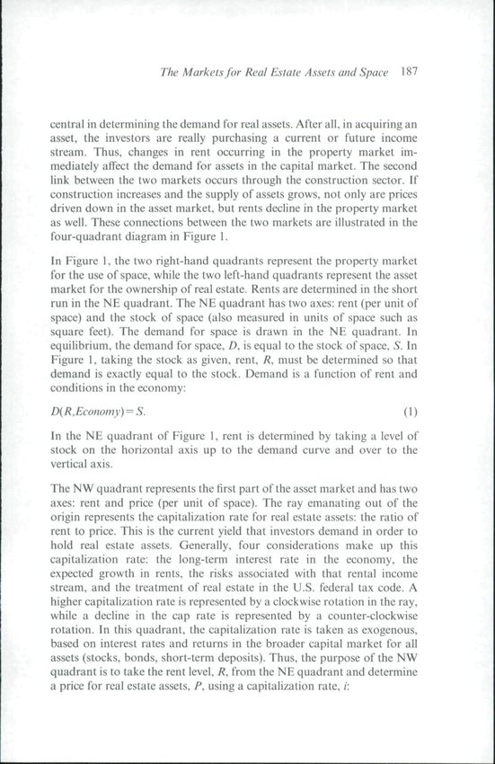
184       Denise DiPasquale and William C. Wheaton

Table 2
Value of U.S. Real Estate, 1990

                                                 Billions              Percent
                                                  of$s                 of Total

Residential                                       6.122                  69.8
  Single-Family Homes                             5,419                  61.7
  Multifamily                                       552                   6.3
  Condominiums/Coops                                 96                   1.1
  Mobile Homes                                       55                   0.6

Retail                                            1,115                  12.7
Office                                            1,009                  11.5
Manufacturing                                       308                   3.5
Warehouse                                           223                   2.5

Total U.S. Real Estate                            8,777                 100.0

Source.    IREM Foundation and Arthur Anderson (1991)

Foundation and Arthur Anderson (1991) has made a gallant attempt at
estimating the value of all U.S. real estate, by type and owner, piecing
together data from a variety of sources. The study employed standard
government statistics, trade association data, and state and county
property tax records to estimate statistically the value of real estate.

In this study, total real estate in the U.S. is estimated to be worth $8.8
trillion. As shown in Table 2, almost 70% of all U.S. real estate is
residential, and almost 90% ofthe value of residential real estate is in the
nation's stock of single-family homes. The 30% of U.S. real estate that is
nonresidential is dominated by office and retail space - at least in dollar
value. Using the Federal Reserve national net worth estimate of $15.6
trillion in 1990, the figures in Table 2 suggest that real estate constitutes
roughly 56% of the nation's wealth.^

- The estimate of national net worth is frotn the Board of Governors (1991). It
should be noted that Ihe Federal Reserve estitnates the value of real estate at $10.7
trillion. Miles argues that the BEA/Federal Reserve estimates of the value of
nonresidential real estate may be high because the data used for the stock estimates
include special purpose fixtures in manufacturing plants which are certainly part of
the nation's capital stock but really should not be included when measuring the
value of real estate (see Miles 1990, p. 74).
The Markets for Real Estate Assets and Space 185

The legal ownership status of this wealth is shown in Table 3. Of
residential real estate, 83% is owned by individuals, including individual
ownership of personal residences and sole proprietor ownership of apart-
ment buildings. The 61.5% of nonresidential real estate that is owned by
corporations covers ownership of investment property as well as buildings
occupied by their corporate owners. Partnerships own almost equal shares
of residential and nonresidentiai property, while corporations dominate
the nonresidential market. Finally, the ownership of U.S. real estate by
foreign entities is virtually nil, despite some considerable concern about
this during the last few years.

In summary, U.S. real estate is the largest component of national wealth,
and the largest component of annual net private investment. This huge
base of assets, however, has been accumulated by devoting only about
5%-7% of each year's GDP to the construction and renovation of that
base. It is, of course, the durability of real estate that allows us to devote
such a small fraction of GDP to the accumulation and maintenance of
such a large share of our assets.

The Markets for Real Estate Assets and Real Estate Space
Since real estate is a durable capital good, its production and price are

Table 3
Who Owns U.S. Real Estate in 1990 (billions of 1990 $s)

                                      AIMReal         Residential    Nonresidential
                                       Estate            Only            Only
                                    Ss    Percent    $s    Percent    $s   Percent

Individuals                         5,088   58.0    5,071    82.8       17     0.6
Corporations                        1,699   19.4       66      1.1   1,633    61.5
Partnerships                        1,011   11.5      673     ll.O     338    12.7
Not-For-Profits                       411    4.7      104     1.7      307    11.6
Government                            234    2.6      173     2.8       61     2.3
Institutional Investors               128    1.5        14    0.2      114     4.3
Financial Institutions                114    1.3        13    0.2      101     3.8
Other (includes foreign)               92    1.0         8    0.1       84     3.2

Total:                              8,777   100.0   6,122    100.0   2,655   100.0
Percent of Alt Real Estate:                 lOO.O            f>9.S            30.2

Source:   IREM Foundation and Arthur Anderson (1991)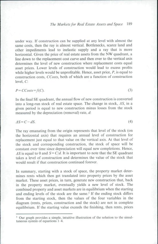
186   Denise DiPasquale and William C. Wheaton

determined in an asset, or capital, market. The price of houses in the U.S.
largely depends on how many households wish to own units and how
many units are available for such ownership. Likewise, the value of
shopping centers depends on how many investors wish to own such space
and how many centers there are available in which to invest. In both cases,
all else equal, an increase in the demand to own these assets will raise
prices while a greater supply of space will depress prices.

The new supply of real estate assets depends on the price of those assets
relative to the cost of replacing or constructing them. In the long run, the
asset market should equate market prices with replacement costs. In the
short run, however, the two may diverge significantly because of the lags
and delays that are inherent in the construction process. For example, if
demand for the ownership of space suddenly rises, then with a fixed
supply of assets, prices will rise as well. With prices now above con-
struction costs, new construction takes piace. As this space arrives on the
market, demand is satisfied and prices begin to fall back towards the cost
of replacement.

In the market for real estate use or space, demand comes from the
occupiers of space, whether they be tenants or owners, firms or house-
holds. For firms, space is one of many factors of production, and like any
other factor, its use will depend on lirm output levels and the relative cost
of space. The household demand for space depends on income and the
cost of occupying that space relative to the cost of consuming other
commodities. For firms or households, the cost of occupying space is the
annual outlay necessary to use real estate - its rent. For tenants, rent is
simply specified in a lease agreement. For owners, rent is defined as the
annuaiized cost associated with the ownership of property.

Rent is determined in the property market for space, not in the asset market
for ownership. In the property market, the supply of space is given from the
asset market. The demand for space depends on rent and other exogenous
economic factors such as firm production levels, income or the number of
households. The task of the property market is to determine a rent level at
which the demand for space equals the supply of space. All else equal, when
the number of households increases or firms expand production, the
demand for space use rises. With fixed supply, rents rise as well.

The link between the markets for assets and property occurs at two
junctions. First, the rent levels determined in the property market are
The Markets for Real Estate Assets and Space       187

central in determining the demand for real assets. After all, in acquiring an
asset, the investors are really purchasing a current or future income
stream. Thus, changes in rent occurring in the property market im-
mediately affect the demand for assets in the capital market. The second
link between the two markets occurs through the construction sector. If
construction increases and the supply of assets grows, not only are prices
driven down in the asset market, but rents decline in the property market
as well. These connections between the two markets are illustrated in the
four-quadrant diagram in Figure 1.

In Figure I, the two right-hand quadrants represent the property market
for the use of space, while the two left-hand quadrants represent the asset
market for the ownership of real estate. Rents are determined in the short
run in the NE quadrant. The NE quadrant has two axes: rent (per unit of
space) and the stock of space (also measured in units of space such as
square feet). The demand for space is drawn in the NF quadrant. In
equilibrium, the demand for space, Z), is equal to the stock of space, S. In
Figure 1, taking the stock as given, rent, R. must be determined so that
demand is exactly equal to the stock. Demand is a function of rent and
conditions in the economy:

D{R.Economy) = S.                                                          (1)

In the NE quadrant of Figure 1, rent is determined by taking a level of
stock on the horizontal axis up to the demand curve and over to the
vertical axis.

The NW quadrant represents the first part of the asset market and has two
axes: rent and price (per unit of space). The ray emanating out of the
origin represents the capitalization rate for real estate assets: the ratio of
rent to price. This is the current yield that investors demand in order to
hold real estate assets. Generally, four considerations make up this
capitalization rate: the long-term interest rate in the economy, the
expected growth in rents, the risks associated with that rental income
stream, and the treatment of real estate in the U.S. federal tax code. A
higher capitalization rate is represented by a clockwise rotation in the ray,
while a decline in the cap rate is represented by a counter-clockwise
rotation. In this quadrant, the capitalization rate is taken as exogenous,
based on interest rates and returns in the broader capital market for all
assets (stocks, bonds, short-term deposits). Thus, the purpose of the NW
quadrant is to take the rent level, R., from the NE quadrant and determine
a price for real estate assets, P, using a capitalization rate, /: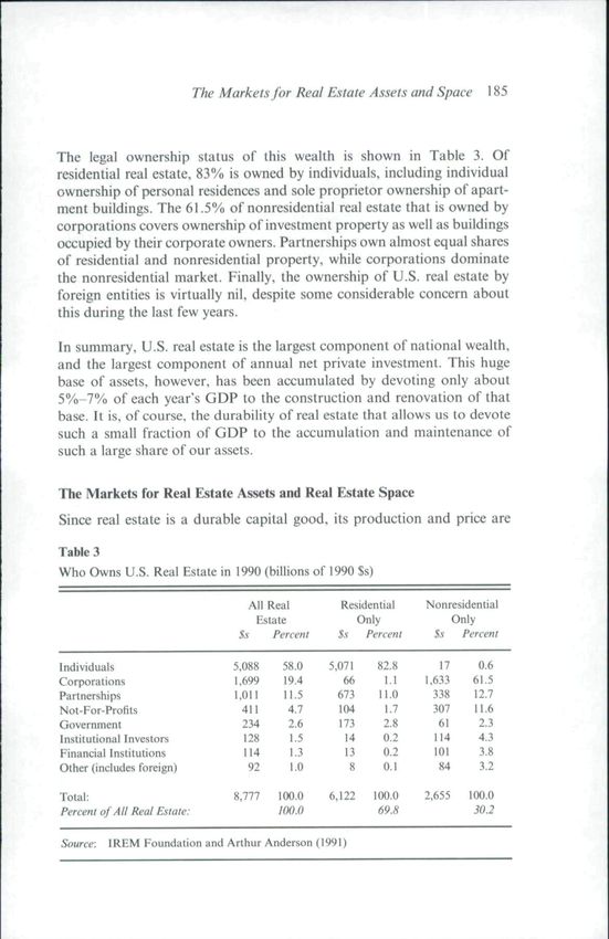
188   Denise DiPasquale and William C. Wheaton

Figure 1
Real Estate: The Property and Asset Markets

A.sset Market:                  Rent                   Property Market:
Valuation                                            Rent Determination

                                                       D{R.Econonn) = S

Price S                                                     Stock (sq ft)

   P-f(C)
  •{P=CCo.sts)

A.s.set Market:              Construction              Property Market:
Construction                   (sq ft)                 Stock Adjusinwnt

                                                                        (2)

In Figure 1, the price of the asset is determined by moving from the rent
level on the vertical axis in the NE quadrant over to the ray in the NW
quadrant, and then down to the horizontal axis (price).

The next (SW) quadrant is that portion of the asset market where the
construction of new assets is determined.

Here, the curve, /(C), represents the replacement cost, CCosts.. of real
estate. In this version of the diagram, the cost of construction is assumed
to increase with greater building activity, and therefore the curve moves in
a southwesterly direction. It intersects the price axis at that minimum
dollar value (per unit of space) required to get some level of construction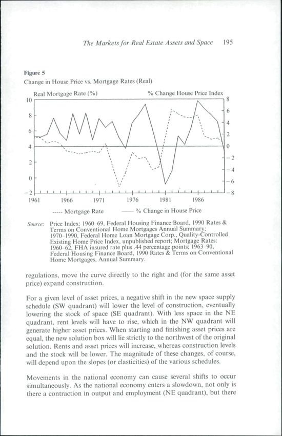
The Markets for Real Estate Assets and Space          189

under way. If construction can be supplied at any level with almost the
same costs, then the ray is almost vertical. Bottlenecks, scarce land and
other impediments lead to inelastic supply and a ray that is more
horizontal. Given the price of real estate assets from the NW quadrant, a
line down to the replacement cost curve and then over to the vertical axis
determines the level of new construction where replacement costs equal
asset prices. Eower levels of construction would lead to excess profits
while higher levels would be unprofitable. Hence, asset price, P, is equal to
construction costs, CCosts, both of which are a function of construction
level, C:

P^ CCosts =f{C).                                                               (3)

In the final SE quadrant, the annual flow of new construction is converted
into a long-run stock of real estate space. The change in stock, ^15, in a
given period is equal to new construction minus losses from the stock
measured by the depreciation (removal) rate, d:

AS=C-dS.                                                                       (4)

The ray emanating from the origin represents that level of the stock (on
the horizontal axis) that requires an annual level of construction for
replacement just equal to that value on the vertical axis. At that level of
the stock and corresponding construction, the stock of space will be
constant over time since depreciation will equal new completions. Hence,
AS is equal to 0 and S^ Cjd. It is important to note that the SE quadrant
takes a level of construction and determines the value of the stock that
would result if that construction continued forever.

In summary, starting with a stock of space, the property market deter-
mines rents which then get translated into property prices by the asset
market. These asset prices, in turn, generate new construction that, back
in the property market, eventually yields a new level of stock. The
combined property and asset markets are in equilibrium when the starting
and ending levels of the stock are the same.^ If the ending stock differs
from the starting stock, then the values of the four variables in the
diagram (rents, prices, construction and the stock) are not in complete
equilibrium. If the starting value exceeds the finishing, then rents, prices

* Our graph provides a simple, intuitive illustration of the solution to the simul-
taneous system of equations 1 4.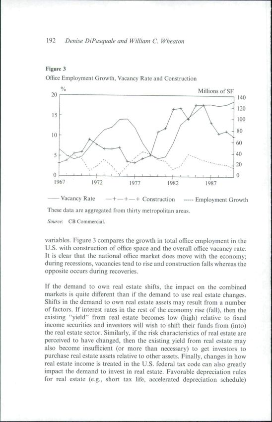
190    Denise DiFasquale and William C. Wheaton

and construction musl all rise to be in equilibrium. If the initial stock is
less than the finishing stock, then rents, prices and construction must
decrease to be in equilibrium.

In the case of real estate occupied by its owner, the four quadrants still
hold, but there are not separate asset and property markets. The deter-
mination of prices and rents occurs with a single decision in a combined
market. In the market for owner-occupied housing, for example, the stock
of single-family homes, the number of households, and their incomes will
determine an annual payment or willingness to pay by those households
who purchase a home (NE quadrant). This is equivalent to a "rent." A
rise in the number of households or a fall in available space means that to
clear the property market, the annual payment to occupy a house must
rise. The NW quadrant then translates this payment into a price actually
paid for the home. Lower interest rates, for example, imply that for the
same annual payment (renl). households can afford to pay a higher
purchase (asset) price. With owner-occupied real estate, a single decision
by the user/owner determines both rent and price. This decision, however,
is influenced by the same economic and capital market conditions as
with rental properties. Once the purchase price is determined, then
construction and eventually the equilibrium stock of space follow in the
other two quadrants (SW.SE).

It is important to realize that the four-quadrant diagram depicts a long-
run equilibrium in the asset and property markets. The diagram is not as
well suited to describing short-run market dynamics or the temporary
disequilibria that often occur in the real estate sector.

Comparative Statics
Using Figure 1, we can trace out the long-run impact of the broader
economy on the real estate market. For illustrative purposes, we consider
the impacts on the real estate market of changes in the macroeconomy
(e.g., growth in income, production, or number of households), short-
term or long-term interest rates, the tax treatment of real estate and the
availability of construction financing. We identify which quadrant initially
is affected by a specific exogenous change and trace the impacts through
the other quadrants.

Increases in employment, production, or the number of households would
increase the demand for space, shifting out the demand curve in the NE
The Markets for Real Estate Assets and Space           191

Figure 2
The Property and Asset Markets: Property Demand Shifts

 Asset Market                   Rent                  Property Market:
 Valuation                                          Rent Determination

                                                         D{ R.Economy) — S

  Price $                                                     Slock (sq ft)

     P=f{C)
     (P= CCosts)                                         JS=C-dS       (5=—)
                                                                              d

  Asset Market:              Construction                Property Market:
  Construction                 (sq ft)                   Stock Adjustment

quadrant. For a given level of real estate space, rents must therefore rise.
These higher rents then lead to greater asset prices in the NW quadrant
which, in turn, generate a higher level of new construction in the SW
quadrant. Eventually this leads to a greater stock of space (SE quadrant).
As shown in Figure 2. the new market equilibrium is the dashed box that
in every direction lies outside of the box that connected the four curves in
the original equilibrium. In the new equilibrium, neither rents, prices,
construction, nor the stock can be less than in the initial equilibrium. The
magnitude of the changes in these variables depends on the slopes of the
various curves. For example, if construction were very elastic with respect
to asset prices, then the new levels of prices and rents would be only
slightly greater than before, whereas construction and stock would
expand considerably.

Economic growth, then, increases all equilibrium variables in the real
estate market, whereas economic contraction leads to decreases in all
192 Denise DiFasquale and William C. Wheaton
Figure 3
Office Employment Growth, Vacancy Rate and Construction
Millions of SF
1967 1972 1977 1982 1987
— Vacancy Rate —+ —+ —-I- Construction -— Employment Growth
These data are aggregated from thirty metropolitan areas.
Source: CB Commercial.
variables. Figure 3 compares the growth in tota! office employment in the
U.S. with construction of office space and the overall office vacancy rate.
It is clear that the national office market does move with the economy;
during recessions, vacancies tend to rise and construction falls whereas the
opposite occurs during recoveries.
If the demand to own real estate shifts, the impact on the combined
markets is quite different than if the demand to use real estate changes.
Shifts in the demand to own real estate assets may result from a number
of factors. If interest rates in the rest of the economy rise (fall), then the
existing "yield" from real estate becomes low (high) relative to fixed
income securities and investors will wish to shift their funds from (into)
the real estate sector. Similarly, if the risk characteristics of real estate are
perceived to have changed, then the existing yield from real estate may
also become insufficient (or more than necessary) to get investors to
purchase real estate assets relative to other assets. Finally, changes in how
real estate income is treated in the U.S. federal tax code can also greatly
impact the demand to invest in real estate. Favorable depreciation rules
for real estate (e.g., short tax life, accelerated depreciation schedule)The Markets for Real Estate Assets and Space 193
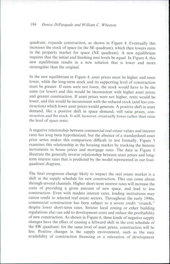
Figure 4
The Property and Asset Markets: Asset Demand Shifts
Asset Market: Rent $ Property Market:
Valuation Rent Determination
D{R.Economy) = S
Price $ Stock (sq ft)
P=f(Q
{P=CCosts) d
Asset Market: Construction Property Market:
Construction (sq ft) Stock Adjustment
increase the after-tax yield generated by real estate. This will increase the
demand to hold real estate assets.
Reductions in long-term interest rates, decreases in the perceived risk of
real estate, and generous depreciation or other favorable changes in the
tax treatment of real estate all will cause a reduction in the income that
investors require from real estate. As shown in Figure 4. in the NW
quadrant, this has the effect of a counter-clockwise rotation in the
capitalization rate ray that emanates out of the origin. Higher interest
rates, greater perceived risk, and adverse tax changes rotate the ray in a
clockwise manner.
Given a level of rent from the property market, a reduction in the current
yield or capitalization rate for real estate raises asset prices and. in the SW194 Denise DiPasquale and William C. Wheaton quadrant, expands construction, as shown in Figure 4. Eventually this increases the stock of space (in the SE quadrant), whieh then lowers rents in the property market for space (NE quadrant). A new equilibrium requires that the initial and finishing rent levels be equal. In Figure 4, this new equilibrium results in a new solution that is lower and more rectangular than the original. In the new equilibrium in Figure 4, asset prices must be higher and rents lower, while the long-term stock and its supporting level of construction must be greater. If rents were not lower, the stock would have to be the same (or lower) and this would be inconsistent with higher asset prices and greater construction. If asset prices were not higher, rents would be lower, and this would be inconsistent with the reduced stock (and less con- struction) which lower asset prices would generate. A positive shift in asset demand, like a positive shift in space demand, will raise prices, con- struction and the stock. It will, however, eventually lower rather than raise the level of space rents. A negative relationship between commercial real estate values and interest rates has long been hypothesized, but the absence of a standardized asset price series makes this comparison difficult to test formally. Figure 5 examines this relationship in the housing market by tracking the historic movements in house prices and mortgage rates. The data in Figure 5 illustrate the generally inverse relationship between asset prices and long- term interest rates that is predicted by the model represented in our four- quadrant diagram. The final exogenous change likely to impact the real estate market is a shift in the supply schedule for new construction. This can come about through several channels. Higher short-term interest rates will increase the costs of providing a given amount of new space, and lead to less construction. Even with modest interest rates, lending institutions may ration credit to selected real estate sectors. Throughout the early 1990s, commercial construction has been subject to a severe credit "crunch," despite lower short-term rates. Stricter local zoning or other building regulations also can add to development costs and reduce the profitability of new construction. As shown in Figure 6, these kinds of negative supply changes have the effect of causing a leftward shift in the cost schedule of the SW quadrant: for the same level of asset prices, construction will be less. Positive changes in the supply environment, such as the easy availability of construction financing or a relaxation of development
The Markets for Real Estate Assets and Space       195

Figure 5
Change in House Price vs. Mortgage Rates (Real)
      Real Mortgage Rale (%)                 % Change House Price Index
 10

                                                                          -8
 1961          1966       1971        1976        1981       1986
                Mortgage Rate            % Change in House Price

 Source: Price Index: 1960-69. Federal Housing Finance Board, 1990 Rates &
         Terms on Conventional Home Mortgages Annual Summary;
         1970 1990, Federal Home Loan Mortgage Corp,, Quality-Controlled
         Existing Home Price Index, unpublished report; Mortgage Rates:
         I960 62, FHA insured rale plus .44 percentage points: 1963 90,
         Federal Housing Finance Board, 1990 Rates & Terms on Conventional
         Home Mortgages, Annual Summary.

regulations, move the curve directly to the right and (for the same asset
price) expand construction.

For a given level of asset prices, a negative shift in the new space supply
schedule (SW quadrant) will lower the level of construction, eventually
lowering the stock of space (SE quadrant). With less space in the NE
quadrant, rent levels will have to rise, which in the NW quadrant will
generate higher asset prices. When starting and finishing asset prices are
equal, the new solution box will lie strictly to the northwest ofthe original
solution. Rents and asset prices will increase, whereas construction levels
and the stock will be lower. The magnitude of these changes, of course,
will depend upon the slopes (or elasticities) ofthe various schedules.

Movements in the national economy can cause several shifts to occur
simultaneously. As the national economy enters a slowdown, not only is
there a contraction in output and employment (NE quadrant), but there
196 Denise DiPasquale and William C. Wheaton
Figure 6
The Property and Asset Markets: Asset Cost Shifts
Asset Market: ReniS Property Market:
Vahiation Rent Determination
D(R.Econimi\) = S
Price Slock (sq ft)
(P=CCosts
Asset Market: Construction Property Market:
Construction (sq ft) Slock Adjusinu'nt
are usually increases in short-term interest rates as well (SW quadrant).
An economic expansion leads to the opposite combination. This com-
bination of shifts can generate any pattern of new box solutions that lies
between the two shown in Figures 2 and 6. Although the analysis gets
more complicated in the case of multiple shifts, the net outcome is always
some combination of the impacts from each individual change.
Conclusions
The distinction between the market for real estate assets and that for real
estate space is an important one as we seek to improve our understanding
of how this major sector operates. To this end, we have presented a simple
analytic framework, illustrated by our four-quadrant diagram, which
highlights this distinction and illustrates how real estate is impacted by
both the nation's macroeconomy and its financial markets. This frame-The Markets for Real Estate Assets and Space 197 work has proven to be very useful in the classroom as a way of introducing students to the operation of the real estate sector. With our four-quadrant analysis, we are able to trace out the impact on rents, asset prices, construction and the stock resulting from various exogenous forces. This simple framework works well in illustrating the new equilibria that result as this exogenous environment changes. An important drawback of this framework is that it is not easy to trace out the intermediate steps as the market moves to its new equilibrium. Depicting the intermediate adjustments ofthe market would require a dynamic system of equations that would significantly complicate our analysis. Developing an intuitive framework similar to the one in this paper that traces the intermediate- term dynamic path to a new equilibrium remains a formidable challenge. This article is based on Chapter I of our hook. The Economics of Real Estate Mdx'&.tXs, forthcoming from Prentice-Halt in 1994. We thank Jean L. Cummings and Henry Pollakowski for helpful comments on an earlier draft. Of course, we are responsible for any errors that remain. References Board of Governors of the Federal Reserve System. 1991. Balance Sheets of the U.S. Economy: 1945-1990. September. 1REM Foundation and Arthur Anderson. 1991. Managing the Future: Real Estate in the 1990s. Miles. M. 1990. What Is the Value of All U.S. Real Estate? Real Estate Review 2(2): 69-77. U.S. Bureau of Census. 1991. Value of New Construction Put in Place: May 1991. Current Construction Reports.
You can also read