The High-Frequency Trading Arms Race: Frequent Batch Auctions as a Market Design Response
←
→
Page content transcription
If your browser does not render page correctly, please read the page content below
The High-Frequency Trading Arms Race: Frequent Batch
                        Auctions as a Market Design Response∗
                               Eric Budish†, Peter Cramton‡, and John Shim§

                                                     February 3, 2015

                                                            Abstract
             The high-frequency trading arms race is a symptom of flawed market design. Instead of
         the continuous limit order book (CLOB) that is currently predominant, we argue that finan-
         cial exchanges should use frequent batch auctions: uniform price double auctions conducted,
         e.g., every tenth of a second. That is, time should be treated as discrete instead of contin-
         uous, and orders should be processed in a batch auction instead of serially. Our argument
         has three parts. First, we use millisecond-level direct-feed data from exchanges to document
         a series of stylized facts about how the CLOB market design works at high-frequency time
         horizons: (i) correlations completely break down; which (ii) leads to obvious mechanical
         arbitrage opportunities; and (iii) competition has not affected the size or frequency of the
         arbitrage opportunities, it has only raised the bar for how fast one has to be to capture them.
         Second, we introduce a simple theory model which is motivated by, and helps explain, the
         empirical facts. The key insight is that obvious mechanical arbitrage opportunities, like those
         observed in the data, are built into the CLOB market design – even symmetrically observed
         public information creates arbitrage rents. These rents harm liquidity provision and induce
         a never-ending socially-wasteful arms race for speed. Last, we show that frequent batch
         auctions directly address the problems caused by the CLOB. Discrete time reduces the value
         of tiny speed advantages, and the auction transforms competition on speed into competition
         on price. Consequently, frequent batch auctions eliminate the mechanical arbitrage rents,
         enhance liquidity for investors, and stop the high-frequency trading arms race.

   ∗
    First version: July 2013. Project start date: Oct 2010. For helpful discussions we are grateful to numerous industry practitioners,
seminar audiences at the University of Chicago, Chicago Fed, Université Libre de Bruxelles, University of Oxford, Wharton, NASDAQ,
IEX Group, Berkeley, NBER Market Design, NYU, MIT, Harvard, Columbia, Spot Trading, CFTC, Goldman Sachs, Toronto, AQR,
FINRA, SEC First Annual Conference on Financial Market Regulation, NBER IO, UK FCA, Northwestern, Stanford, Netherlands
AFM, and to Susan Athey, Larry Ausubel, Eduardo Azevedo, Simcha Barkai, Ben Charoenwong, Adam Clark-Joseph, John Cochrane,
Doug Diamond, Darrell Duffie, Gene Fama, Doyne Farmer, Thierry Foucault, Alex Frankel, Matt Gentzkow, Larry Glosten, Terry
Hendershott, Ali Hortacsu, Laszlo Jakab, Emir Kamenica, Brian Kelly, Pete Kyle, Jon Levin, Donald MacKenzie, Gregor Matvos,
Albert Menkveld, Paul Milgrom, Toby Moskowitz, Matt Notowidigdo, Mike Ostrovsky, David Parkes, Canice Prendergast, Al Roth,
Gideon Saar, Jesse Shapiro, Spyros Skouras, Andy Skrzypacz, Chester Spatt, Lars Stole, Geoff Swerdlin, Richard Thaler, Brian Weller,
Michael Wellman and Bob Wilson. We thank Daniel Davidson, Michael Wong, Ron Yang, and especially Geoff Robinson for outstanding
research assistance. Budish gratefully acknowledges financial support from the National Science Foundation (ICES-1216083), the Fama-
Miller Center for Research in Finance at the University of Chicago Booth School of Business, and the Initiative on Global Markets at
the University of Chicago Booth School of Business.
   †
       Corresponding author. University of Chicago Booth School of Business, eric.budish@chicagobooth.edu
   ‡
       University of Maryland, pcramton@gmail.com
   §
       University of Chicago Booth School of Business, john.shim@chicagobooth.edu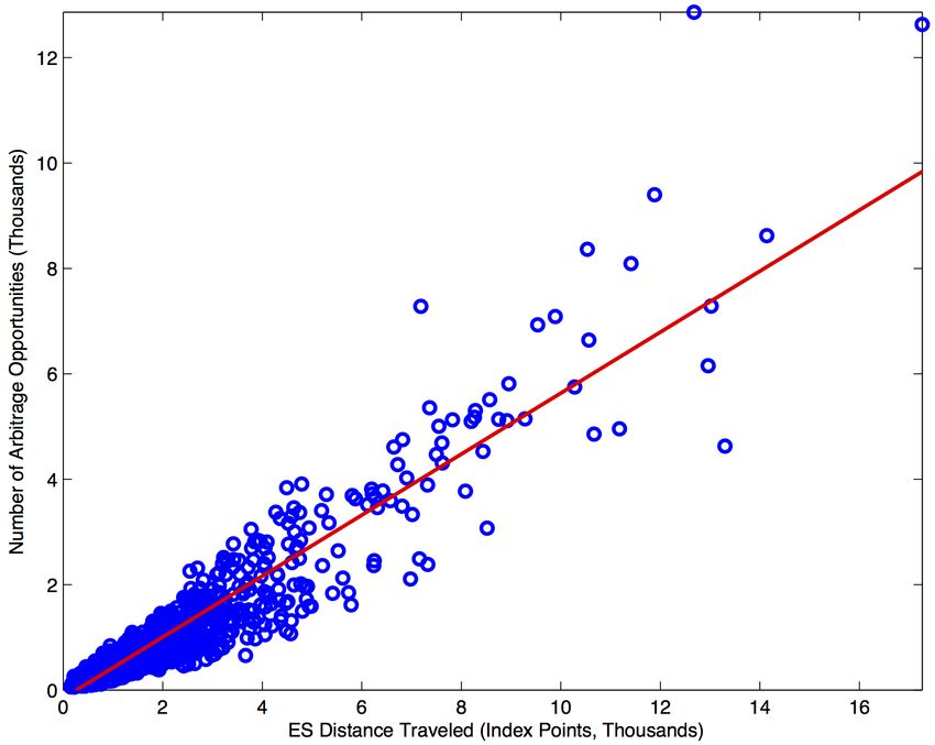
1

1         Introduction
In 2010, Spread Networks completed construction of a new high-speed fiber optic cable connecting
financial markets in New York and Chicago. Whereas previous connections between the two
financial centers zigzagged along railroad tracks, around mountains, etc., Spread Networks’ cable
was dug in a nearly straight line. Construction costs were estimated at $300 million. The result
of this investment? Round-trip communication time between New York and Chicago was reduced
. . . from 16 milliseconds to 13 milliseconds. 3 milliseconds may not seem like much, especially
relative to the speed at which fundamental information about companies and the economy evolves.
(The blink of a human eye lasts 400 milliseconds; reading this parenthetical took roughly 3000
milliseconds.) But industry observers remarked that 3 milliseconds is an “eternity” to high-
frequency trading (HFT) firms, and that “anybody pinging both markets has to be on this line,
or they’re dead.” One observer joked at the time that the next innovation will be to dig a tunnel,
speeding up transmission time even further by “avoiding the planet’s pesky curvature.” Spread
Networks may not find this joke funny anymore, as its cable is already obsolete. While tunnels
have yet to materialize, a different way to get a straighter line from New York to Chicago is to use
microwaves rather than fiber optic cable, since light travels faster through air than glass. Since
its emergence in around 2011, microwave technology has reduced round-trip transmission time
first to around 10ms, then 9ms, then 8.5ms, and most recently to 8.1ms. Analogous speed races
are occurring throughout the financial system, sometimes measured at the level of microseconds
(millionths of a second) and even nanoseconds (billionths of a second).1
        We argue that the high-frequency trading arms race is a symptom of a basic flaw in financial
market design: continuous-time trading. That is, under the continuous limit order book (CLOB)
market design that is currently predominant, it is possible to buy or sell stocks or other securities
at any instant during the trading day.2 We propose a simple alternative: discrete-time trading.
More precisely, we propose a market design in which the trading day is divided into extremely
frequent but discrete time intervals, of length, say, 100 milliseconds. All trade requests received
during the same interval are treated as having arrived at the same (discrete) time. Then, at the
end of each interval, all outstanding orders are processed in batch, using a uniform-price auction,
    1
     Sources for this paragraph: “Wall Street’s Speed War,” Forbes, Sept 27th 2010; “The Ultimate Trading
Weapon,” ZeroHedge.com, Sept 21st 2010; “Wall Street’s Need for Trading Speed: The Nanosecond Age,” Wall
Street Journal, June 2011; “Networks Built on Milliseconds,” Wall Street Journal, May 2012; “Raging Bulls: How
Wall Street Got Addicted to Light-Speed Trading,” Wired, Aug 2012; “CME, Nasdaq Plan High-Speed Network
Venture,” Wall Street Journal March 2013; “Information Transmission between Financial Markets in Chicago and
New York” by Laughlin et al (2014); McKay Brothers Microwave latency table, Jan 20th 2015, Aurora-Carteret
route.
   2
     Computers do not literally operate in continuous time; they operate in discrete time in increments of about
0.3 nanoseconds. More precisely what we mean by continuous time is as-fast-as-possible discrete time plus random
serial processing of orders that reach the exchange at the exact same discrete time.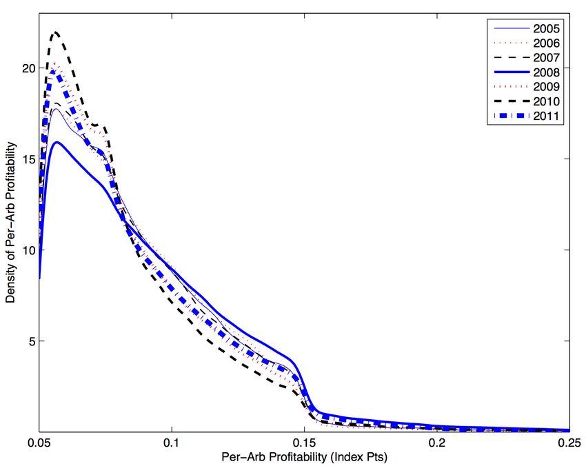
2

as opposed to the serial processing that occurs in the continuous market. We call this market
design frequent batch auctions. Our argument against continuous limit order books and in favor
of frequent batch auctions has three parts.
       The first part of our paper uses millisecond-level direct-feed data from exchanges to document
a series of stylized facts about the CLOB market design. Together, the facts suggest that the
CLOB market design violates basic asset pricing principles at high-frequency time horizons; that
is, the continuous-time market does not actually “work” in continuous time. Consider Figure
1.1. The figure depicts the price paths of the two largest securities that track the S&P 500
index, the SPDR S&P 500 exchange traded fund (ticker SPY) and the S&P 500 E-mini futures
contract (ticker ES), on a trading day in 2011. In Panel A, we see that the two securities are nearly
perfectly correlated over the course of the trading day, as we would expect given the near-arbitrage
relationship between them. Similarly, the securities are nearly perfectly correlated over the course
of an hour (Panel B) or a minute (Panel C). However, when we zoom in to high-frequency time
scales, in Panel D, we see that the correlation breaks down. Over all trading days in 2011, the
median return correlation is just 0.1016 at 10 milliseconds and 0.0080 at 1 millisecond.3 This
correlation breakdown in turn leads to obvious mechanical arbitrage opportunities, available to
whomever is fastest. For instance, at 1:51:39.590 pm, after the price of ES has just jumped roughly
2.5 index points, the arbitrage opportunity is to buy SPY and sell ES.
       The usual economic intuition about obvious arbitrage opportunities is that, once discovered,
competitive forces eliminate the inefficiency. But that is not what we find here. Over the time
period of our data, 2005-2011, we find that the duration of ES-SPY arbitrage opportunities declines
dramatically, from a median of 97ms in 2005 to a median of 7ms in 2011. This reflects the
substantial investments by HFT firms in speed during this time period. But we also find that the
profitability of ES-SPY arbitrage opportunities is remarkably constant throughout this period, at
a median of about 0.08 index points per unit traded. The frequency of arbitrage opportunities
varies considerably over time, but its variation is driven almost entirely by variation in market
volatility. These findings suggest that while there is an arms race in speed, the arms race does
not actually affect the size of the arbitrage prize; rather, it just continually raises the bar for how
fast one has to be to capture a piece of the prize. A complementary finding is that the number
of milliseconds necessary for economically meaningful correlations to emerge has been steadily

   3
     There are some subtleties involved in calculating the 1 millisecond correlation between ES and SPY, since
it takes light roughly 4 milliseconds to travel between Chicago (where ES trades) and New York (where SPY
trades), and this represents a lower bound on the amount of time it takes information to travel between the two
markets (Einstein, 1905). Whether we compute the correlation based on New York time (treating Chicago events
as occurring 4ms later in New York than they do in Chicago), based on Chicago time, or ignore the theory of
special relativity and use SPY prices in New York time and ES prices in Chicago time, the correlation remains
essentially zero. See Section 5 and Appendix B.1 for further details.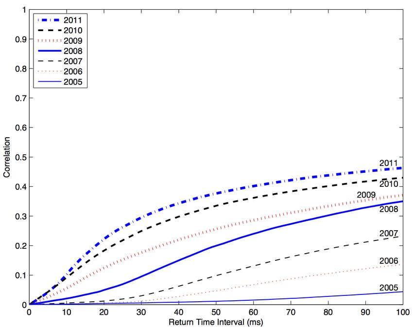
3
Figure 1.1: ES and SPY Time Series at Human-Scale and High-Frequency Time Horizons
Notes: This figure illustrates the time series of the E-mini S&P 500 future (ES) and SPDR S&P 500 ETF (SPY)
bid-ask midpoints over the course of a trading day (Aug 9, 2011) at different time resolutions: the full day (a),
an hour (b), a minute (c), and 250 milliseconds (d). SPY prices are multiplied by 10 to reflect that SPY tracks
1
10 the S&P 500 Index. Note that there is a difference in levels between the two securities due to differences in
cost-of-carry, dividend exposure, and ETF tracking error; for details see Section 5.2.1. For details regarding the
data, see Section 4.
(a) Day (b) Hour
1170 1180
ES Midpoint ES Midpoint
SPY Midpoint SPY Midpoint
1160 1170
1140 1150
1150 1160
1130 1140
1140 1150
Index Points (SPY)
Index Points (SPY)
Index Points (ES)
Index Points (ES)
1130 1140 1120 1130
1120 1130
1110 1120
1110 1120
1100 1110
1100 1110
1090 1100
09:00:00 10:00:00 11:00:00 12:00:00 13:00:00 14:00:00 13:30:00 13:45:00 14:00:00 14:15:00 14:30:00
Time (CT) Time (CT)
(c) Minute (d) 250 Milliseconds
ES Midpoint ES Midpoint
SPY Midpoint SPY Midpoint
1120 1126
1120 1126
1118 1124
Index Points (SPY)
Index Points (SPY)
Index Points (ES)
Index Points (ES)
1119 1125
1116 1122
1118 1124
1114 1120
1117 1123
13:51:00 13:51:15 13:51:30 13:51:45 13:52:00 13:51:39.500 13:51:39.550 13:51:39.600 13:51:39.650 13:51:39.700 13:51:39.750
Time (CT) Time (CT)4
decreasing over the time period 2005-2011; but, in all years, correlations are essentially zero at
high-enough frequency. Overall, our analysis suggests that the mechanical arbitrage opportunities
and resulting arms race should be thought of as a constant of the market design, rather than as
an inefficiency that is competed away over time.
We compute that the total prize at stake in the ES-SPY race averages $75 million per year.
And, of course, ES-SPY is just a single pair of securities – there are hundreds if not thousands
of other pairs of highly correlated securities, and, in fragmented equity markets, arbitrage trades
that are even simpler, since the same stock trades on multiple venues. While we hesitate to put a
precise estimate on the total size of the prize in the speed race, common sense extrapolation from
our ES-SPY estimates suggests that the sums are substantial.
The second part of our paper presents a simple new theory model which is motivated by, and
helps to explain and interpret, these empirical facts. The model serves as a critique of the CLOB
market design, and it also articulates the economics of the HFT arms race. In the model, there
is a security, x, that trades on a CLOB market, and a public signal of x’s value, y. We make a
purposefully strong assumption about the relationship between x and y: the fundamental value
of x is perfectly correlated to the public signal y. Moreover, we assume that x can always be
costlessly liquidated at its fundamental value, and, initially, assume away all latency for trading
firms (aka HFTs, market makers, algorithmic traders). This setup can be interpreted as a “best
case” scenario for price discovery and liquidity provision in a CLOB, assuming away asymmetric
information, inventory costs, etc.
Given that we have eliminated the traditional sources of costly liquidity provision, one might
expect that Bertrand competition among trading firms leads to costless liquidity for investors and
zero rents for trading firms. But, consider the mechanics of what happens in the CLOB market
for x when the public signal y jumps – the moment at which the correlation between x and y
temporarily breaks down. For instance, imagine that x represents SPY and y represents ES, and
consider what happens at 1:51:39.590 pm in Figure 1.1 Panel D, when the price of ES has just
jumped. At this moment, trading firms providing liquidity in the market for x will send a message
to the exchange to adjust their quotes – cancel their stale quotes and replace them with updated
quotes based on the new value of y . At the exact same time, however, other trading firms will try
to “snipe” the stale quotes – send a message to the exchange attempting to buy x at the old ask,
before the liquidity providers can adjust. Since the CLOB processes message requests in serial
(i.e., one at a time in order of receipt), it is effectively random whose request is processed first.
And, to avoid being sniped, each one liquidity provider’s request to cancel has to get processed
before all of the other trading firms’ requests to snipe her stale quotes; hence, if there are N
N −1
trading firms, each liquidity provider is sniped with probability N
. This shows that trading5
firms providing liquidity, even in an environment with only symmetric information and with no
latency, still get sniped with high probability because of the rules of the CLOB market design.
The obvious mechanical arbitrage opportunities we observed in the data are in a sense “built in”
to the CLOB: even symmetrically observed public information creates arbitrage rents.
These arbitrage rents increase the cost of liquidity provision. In a competitive market, trading
firms providing liquidity incorporate the cost of getting sniped into the bid-ask spread that they
charge; so, there is a positive bid-ask spread even without asymmetric information about funda-
mentals. Similarly, sniping causes CLOB markets to be thin; that is, it is especially expensive for
investors to trade large quantities of stock. The reason is that sniping costs scale linearly with
the quantity liquidity providers offer in the book – if quotes are stale, they will get sniped for the
whole amount. Whereas, the benefits of providing a deep book scale less than linearly – since only
some investors wish to trade large amounts.4,5
These arbitrage rents also induce a never-ending speed race. We modify our model to allow
trading firms to invest in a simple speed technology, which allows them to observe innovations in
y faster than trading firms who do not invest. With this modification, the arbitrage rents lead to
a classic prisoner’s dilemma: snipers invest in speed to try to win the race to snipe stale quotes;
liquidity providers invest in speed to try to get out of the way of the snipers; and all trading
firms would be better off if they could collectively commit not to invest in speed, but it is in
each firm’s private interest to invest. Notably, competition in speed does not fix the underlying
problem of mechanical arbitrages from symmetrically observed public information. The size of
the arbitrage opportunity, and hence the harm to investors via reduced liquidity, depends neither
on the magnitude of the speed improvements (be they milliseconds, microseconds, nanoseconds,
etc.), nor on the cost of cutting edge speed technology (if speed costs get smaller over time there
is simply more entry). The arms race is thus an equilibrium constant of the CLOB market design
– a result which ties in closely with our empirical findings.
4
Our source of costly liquidity provision should be viewed as incremental to the usual sources of costly liquidity
provision: inventory costs (Demsetz, 1968; Stoll, 1978), asymmetric information (Copeland and Galai, 1983; Glosten
and Milgrom, 1985; Kyle, 1985), and search costs (Duffie, Garleanu and Pedersen, 2005). Mechanically, our source
of costly liquidity provision is most similar to that in Copeland and Galai (1983) and Glosten and Milgrom (1985)
– we discuss the relationship in detail in Section 6.3. Note too that while our model is extremely stylized, one
thing we do not abstract from is the rules of the CLOB market design itself, whereas Glosten and Milgrom (1985)
and subsequent market microstructure analyses of limit order book markets use a discrete-time sequential-move
modeling abstraction of the CLOB. This abstraction is innocuous in the context of these prior works, but it
precludes a race to respond to symmetrically observed public information as in our model.
5
A point of clarification: our claim is not that markets are less liquid today than before the rise of electronic
trading and HFT; the empirical record is clear that trading costs are lower today than in the pre-HFT era, though
most of the benefits appear to have been realized in the late 1990s and early 2000s (cf. Virtu, 2014, pg. 103; Angel,
Harris and Spatt, 2013, pg. 23; and Frazzini, Israel and Moskowitz, 2012, Table IV). Rather, our claim is that
markets are less liquid today than they would be under an alternative market design that eliminated sniping. For
further discussion see Section 6.5.4.6
The third and final part of our paper shows that the frequent batch auction market design
directly addresses the problems we have identified with the CLOB market design. Frequent batch
auctions may sound like a very different market design from the CLOB, but there are really
just two differences. First, time is treated as discrete instead of continuous.6 Second, orders are
processed in batch instead of serial – since multiple orders can arrive at the same (discrete) time
– using a standard uniform-price auction. All other design details are similar to the CLOB. For
instance, orders consist of price, quantity and direction, and can be canceled or modified at any
time; priority is price then (discrete) time; there is a well-defined bid-ask spread; and information
policy is analogous: orders are received by the exchange, processed by the exchange (at the end
of the discrete time interval, as opposed to continuously), and only then announced publicly.
Together, the two key design differences – discrete-time, and batch processing using an auction
– have two beneficial effects. First, they substantially reduce the value of a tiny speed advantage,
which eliminates the arms race. In the continuous-time market, if one trader is even 100 microsec-
onds faster than the next then any time there is a public price shock the faster trader wins the
race to respond. In the discrete-time market, such a small speed advantage almost never matters.
δ
Formally, if the batch interval is τ , then a δ speed advantage is only τ
as likely to matter as in
the continuous-time market. So, if the batch interval is 100 milliseconds, then a 100 microsecond
1
speed advantage is 1000
as important. Second, and more subtly, the auction eliminates sniping, by
transforming the nature of competition. In the CLOB market design, it is possible to earn a rent
based on a piece of information that many traders observe at basically the same time, because
CLOBs process orders in serial, and somebody is always first. In the frequent batch auction mar-
ket, by contrast, if multiple traders observe the same information at the same time, they are forced
to compete on price instead of speed. It is no longer possible to earn a rent from symmetrically
observed public information.
For both of these reasons, frequent batch auctions eliminate the purely mechanical cost of
liquidity provision in CLOB markets associated with stale quotes getting sniped. Intuitively,
discrete time reduces the likelihood that a tiny speed advantage yields asymmetric information,
and the auction ensures that symmetric information does not generate arbitrage rents. Batching
also resolves the prisoner’s dilemma associated with the CLOB market design, and in a manner
that allocates the welfare savings to investors. In equilibrium, relative to the CLOB, frequent
batch auctions eliminate sniping, enhance liquidity, and stop the HFT arms race.
We emphasize that the market design perspective we take in this paper sidesteps the “is HFT
good or evil?” debate which seems to animate much of the current discussion about HFT among
6
This paper does not characterize a specific optimal batch interval. See Section 7.4 and Appendix C.2 for a
discussion of what the present paper’s analysis does and does not teach us about the optimal batch interval.7
policy makers, the press, and market microstructure researchers. The market design perspective
assumes that market participants optimize with respect to market rules as given, but takes seriously
the possibility that the rules themselves are flawed. Many of the negative aspects of HFT which
have garnered so much public attention are best understood as symptoms of flawed market design.
However, the policy ideas that have been most prominent in response to concerns about HFT –
e.g., Tobin taxes, minimum resting times, message limits – attack symptoms rather than address
the root market design flaw: continuous-time, serial-process trading. Frequent batch auctions
directly address the root flaw.
The rest of the paper is organized as follows. Section 2 discusses related literature. Section
3 briefly reviews the rules of the continuous limit order book. Section 4 describes our direct-feed
data from NYSE and the CME. Section 5 presents the empirical results on correlation break-
down and mechanical arbitrage. Section 6 presents the model, and solves for and discusses the
equilibrium of the CLOB. Section 7 analyzes frequent batch auctions, shows why they directly
address the problems with the CLOB, and discusses their equilibrium properties. Section 8 dis-
cusses computational advantages of discrete-time trading over continuous-time trading. Section
9 concludes. Supporting materials are contained in a series of appendices. Appendix A uses our
model to discuss alternative responses to the HFT arms race, including Tobin taxes, random de-
lays, asymmetric delays, and minimum resting times. Appendix B provides backup materials for
the empirical analysis. Appendix C provides backup materials for the theoretical analysis.
2 Related Literature
First, there is a well-known older academic literature on infrequent batch auctions, e.g., three
times per day (opening, midday, and close). Important contributions to this literature include
Cohen and Schwartz (1989); Madhavan (1992); Economides and Schwartz (1995); see also Schwartz
(2001) for a book treatment. We emphasize that the arguments for infrequent batch auctions in
this earlier literature are completely distinct from the arguments we make for frequent batch
auctions. Our argument focuses on eliminating sniping, encouraging competition on price rather
than speed, and stopping the arms race. The earlier literature focused on enhancing the accuracy
of price discovery by aggregating the dispersed information of investors into a single price,7 and
on reducing intermediation costs by enabling investors to trade with each other directly. Perhaps
the simplest way to think about the relationship between our work and this earlier literature is as
7
In Economides and Schwartz (1995), the aggregation is achieved by conducting the auction at three significant
points during the trading day (opening, midday, and close). In Madhavan (1992) the aggregation is achieved by
waiting for a large number of investors with both private- and common-value information to arrive to market.8
follows. Our work shows that there is a discontinuous welfare and liquidity benefit from moving
from continuous time to discrete time; more precisely, from the continuous-time serial-process
CLOB to discrete-time batch-process auctions. The earlier literature then suggests that there
might be additional further benefits to greatly lengthening the batch interval that are outside
our model. But, there are also likely to be important costs to such lengthening that are outside
our model, and that are outside the models of this earlier literature as well. Developing a richer
understanding of the costs of lengthening the time between auctions is an important topic for
future research.
We also note that our specific market design details differ from those in this earlier literature,
beyond simply the frequency with which the auctions are conducted. Differences include informa-
tion policy, the treatment of unexecuted orders, and time priority rules; see Section 7.1 for a full
description.
Second, there are two recent papers, developed independently and contemporaneously8 from
ours and coming from different methodological perspectives, that also make cases for frequent batch
auctions. Closest in spirit is Farmer and Skouras (2012), a non-formal policy paper commissioned
by the UK Government’s Foresight Report. They, too, argue that continuous trading leads to
an arms race for speed, and that frequent batch auctions stop the arms race. There are three
substantive differences between our arguments. First, two conceptually important ideas that
come out of our formal model are that arbitrage rents are built in to the CLOB market design,
in the sense that even symmetrically observed public information creates arbitrage opportunities
due to serial processing, and that the auction eliminates these rents by transforming competition
on speed into competition on price. These two ideas are not identified in Farmer and Skouras
(2012). Second, the details of our proposed market designs are substantively different. Our theory
identifies the key flaws of the CLOB and shows that these flaws can be corrected by modifying
only two things: time is treated as discrete instead of continuous, and orders are processed in
batch using an auction instead of serially. Farmer and Skouras (2012) departs more dramatically
from the CLOB, demarcating time using an exponential random variable and entirely eliminating
time-based priority.9 Last, a primary concern of Farmer and Skouras (2012) is market stability,
a topic we touch on only briefly in Section 8. Wah and Wellman (2013) make a case for frequent
batch auctions using a zero-intelligence (i.e., non-game theoretic) agent-based simulation model.
In their simulation model, investors have heterogeneous private values (costs) for buying (selling)
8
We began work on this project in October 2010.
9
There have been several other white papers and essays making cases for frequent batch auctions, which to
our knowledge were developed independently and roughly contemporaneously: Cinnober (2010); Sparrow (2012);
McPartland (2013); ISN (2013); Schwartz and Wu (2013). In each case, the proposed market design either departs
more dramatically from the CLOB than ours or there are important design details that are omitted.9 a unit of a security, and use a mechanical strategy of bidding their value (or offering at their cost). Batch auctions enhance efficiency in their setup by aggregating supply and demand and executing trades at the market-clearing price. Note that this is a similar argument in favor of frequent batch auctions as that associated with the older literature on infrequent batch auctions referenced above. The reason that this force pushes towards frequent batch auctions in Wah and Wellman (2013) is that their simulations utilize an extremely high discount rate of 6 basis points per millisecond. Third, our paper relates to the burgeoning academic literature on high-frequency trading; see Jones (2013); Biais and Foucault (2014); O’Hara (2015) for recent surveys. One focus of this literature has been on the empirical study of the effect of high-frequency trading on market quality, within the context of the current market design. Examples include Hendershott, Jones and Menkveld (2011); Brogaard, Hendershott and Riordan (2014a,b); Hasbrouck and Saar (2013); Foucault, Kozhan and Tham (2014); Menkveld and Zoican (2014). We discuss the relationship between our results and aspects of this literature in Section 6.5.4. Biais, Foucault and Moinas (2013) study the equilibrium level of investment in speed technology in the context of a Grossman- Stiglitz style rational expectations model. They find that investment in speed can be socially excessive, as we do in our model, and argue for a Pigovian tax on speed technology as a policy response. The Nasdaq “SOES Bandits” were an early incarnation of stale-quote snipers, in the context of an electronic market design that had an unusual feature – the prohibition of automated quote updates – that was exploited by the bandits. See Foucault, Roell and Sandas (2003) for a theoretical analysis and Harris and Schultz (1998) for empirical facts. Further discussion of other related work from this literature is incorporated into the body of the paper. Fourth, our paper is in the tradition of the academic literature on market design. This literature focuses on designing the “rules of the game” in real world markets to achieve objectives such as economic efficiency. Examples of markets that have been designed by economists include auction markets for wireless spectrum licenses and the market for matching medical school graduates to residency positions. See Klemperer (2004) and Milgrom (2004, 2011) for surveys of the market design literature on auction markets and Roth (2002, 2008) for surveys on the market design literature on matching markets. Some papers in this literature that are conceptually related to ours, albeit focused on different market settings, are Roth and Xing (1994) on the timing of transactions, Roth and Xing (1997) on serial versus batch processing, and Roth and Ockenfels (2002) on bid sniping. Last, several of the ideas in our critique of the CLOB market design are new versions of classical ideas. Correlation breakdown is an extreme version of a phenomenon first documented by Epps (1979); see Section 5 for further discussion. Sniping, and its negative effect on liquidity, is closely related to Glosten and Milgrom (1985) adverse selection; see Section 6.3 which discusses this
10

relationship in detail. The idea that financial markets can induce inefficient speed competition
traces at least to Hirshleifer (1971); in fact, our model clarifies that in a CLOB fast traders can
earn a rent even from information that they observe at exactly the same time as other fast traders,
which can be viewed as the logical extreme of what Hirshleifer (1971) called “foreknowledge” rents.

3     Brief Description of Continuous Limit Order Books
In this section we summarize the rules of the continuous limit order book (CLOB) market design.
Readers familiar with these rules can skip this section. Readers interested in further details should
consult Harris (2002).
    The basic building block of this market design is the limit order. A limit order specifies a price,
a quantity, and whether the order is to buy or to sell, e.g., “buy 100 shares of XYZ at $100.00”.
Traders may submit limit orders to the market at any time during the trading day, and they may
also fully or partially withdraw their outstanding limit orders at any time.
    The set of limit orders outstanding at any particular moment is known as the limit order book.
Outstanding orders to buy are called bids and outstanding orders to sell are called asks. The
difference between the best (highest) bid and the best (lowest) ask is known as the bid-ask spread.
    Trade occurs whenever a new limit order is submitted that is either a buy order with a price
weakly greater than the current best ask or a sell order with a price weakly smaller than the current
best bid. In this case, the new limit order is interpreted as either fully or partially accepting one
or more outstanding asks. Orders are accepted in order of the attractiveness of their price, with
ties broken based on which order has been in the book the longest; this is known as price-time
priority. For example, if there are outstanding asks to sell 1000 shares at $100.01 and 1000 shares
at $100.02, a limit order to buy 1500 shares at $100.02 (or greater) would get filled by trading all
1000 shares at $100.01, and then by trading the 500 shares at $100.02 that have been in the book
the longest. A limit order to buy 1500 shares at $100.01 would get partially filled, by trading 1000
shares at $100.01, with the remainder of the order remaining outstanding in the limit order book
(500 shares at $100.01).
    Observe that order submissions and order withdrawals are processed by the exchange in serial,
that is, one-at-a-time in order of their receipt. This serial-processing feature of the continuous
limit order book plays an important role in the theoretical analysis in Section 6.
    In practice, there are many other order types that traders can use in addition to limit orders.
These include market orders, stop-loss orders, fill-or-kill, and dozens of others that are considerably
more obscure (e.g., Patterson and Strasburg, 2012; Nanex, 2012). These alternative order types
are ultimately just proxy instructions to the exchange for the generation of limit orders. For
11
instance, a market order is an instruction to the exchange to place a limit order whose price is
such that it executes immediately, given the state of the limit order book at the time the message
is processed.
4 Data
We use “direct-feed” data from the Chicago Mercantile Exchange (CME) and New York Stock
Exchange (NYSE). Direct-feed data record all activity that occurs in an exchange’s limit order
book, message by message, with millisecond resolution timestamps assigned to each message by
the exchange at the time the message is processed.10 Practitioners who demand the lowest latency
data (e.g. high-frequency traders) use this direct-feed data in real time to construct the limit order
book.
The CME dataset is called CME Globex DataMine Market Depth. Our data cover all limit
order book activity for the E-mini S&P 500 Futures Contract (ticker ES) over the period of Jan 1,
2005 - Dec 31, 2011. The NYSE dataset is called TAQ NYSE ArcaBook. While this data covers
all US equities traded on NYSE, we focus most of our attention on the SPDR S&P 500 exchange
traded fund (ticker SPY). Our data cover the period of Jan 1, 2005 - Dec 31, 2011, with the
exception of a three-month gap from 5/30/2007-8/28/2007 resulting from data issues acknowledged
to us by the NYSE data team. We also drop, from both datasets, the Thursday and Friday from
the week prior to expiration for every ES expiration month (March, June, September, December)
due to the rolling over of the front month contract, half days (e.g., day after Thanksgiving), and a
small number of days in which either dataset’s zip file is corrupted or truncated. We are left with
1560 trading days in total.
Each message in direct-feed data represents a change in the order book at that moment in time.
It is the subscriber’s responsibility to construct the limit order book from this feed, maintain the
status of every order in the book, and update the internal limit order book based on incoming
messages. In order to interpret raw data messages reported from each feed, we write a feed parser
for each raw data format and update the state of the order book after every new message.11
We emphasize that direct feed data are distinct from the so-called “regulatory feeds” provided
by the exchanges to market regulators. In particular, the TAQ NYSE ArcaBook dataset is distinct
from the more familiar TAQ NYSE Daily dataset (sometimes simply referred to as TAQ), which is
an aggregation of orders and trades from all Consolidated Tape Association exchanges. The TAQ
10
Prior to Nov 2008, the CME datafeed product did not populate the millisecond field for timestamps, so the
resolution was actually centisecond not millisecond. CME recently announced that the next iteration of its datafeed
product will be at microsecond resolution.
11
Our feed parsers will be made publicly available in the data appendix.12
data is comprehensive in regards to trades and quotes listed at all participant exchanges, which
includes the major electronic exchanges BATS, NASDAQ, and NYSE and also small exchanges
such as the Chicago Stock Exchange. However, regulatory feed data have time stamps that are
based on the time at which the data are provided to the consolidated feed, and practitioners
estimate that the TAQ’s timestamps were substantially delayed relative to the direct-feed data
that comes directly from the exchanges (our own informal comparisons confirm this; see also Ding,
Hanna and Hendershott (2014)). One source of delay is that the TAQ’s timestamps do not come
directly from the exchanges’ order matching engines. A second source of delay is the aggregation
of data from several different exchanges, with the smaller exchanges considered especially likely
to be a source of delay. The key advantage of our direct-feed data is that the time stamps are
as accurate as possible. In particular, these are the same data that HFT firms subscribe to and
process in real time to make trading decisions.
5 Correlation Breakdown and Mechanical Arbitrage
In this section we report two sets of stylized facts about how continuous limit order book markets
behave at high-frequency time horizons. First, we show that correlations completely break down
at high-enough frequency. Second, we show that there are frequent mechanical arbitrage oppor-
tunities associated with this correlation breakdown, which are available to whichever trader acts
fastest.
For each result we first present summary statistics and then explore how the phenomenon
has evolved over the time-period of our data, 2005-2011. The summary statistics give a sense of
magnitudes for what we depicted anecdotally in Figure 1.1. The time-series evidence explores how
the pattern depicted in Figure 1.1 has evolved over time.
Before proceeding, we emphasize that the finding that correlations break down at high-enough
frequency – which is an extreme version of a phenomenon discovered by Epps (1979)12 – is obvious
from introspection alone, at least ex-post. There is nothing in current market architecture – in
which each security trades in continuous time on its own separate limit-order book, rather than
in a single combinatorial auction market – that would allow different securities’ prices to move
at exactly the same time. It is only when we show that correlation breakdown is associated with
frequent mechanical arbitrage opportunities that we can interpret it as a meaningful issue rather
than a theoretical curiosity.
12
Epps (1979) found that equity market correlations among stocks in the same industry (e.g., Ford-GM) were
much lower over short time intervals than over longer time intervals; in that era, “very short” meant ten minutes,
and long meant a few days.13
Figure 5.1: ES and SPY Correlation by Return Interval: 2011
Notes: This figure depicts the correlation between the return of the E-mini S&P 500 future (ES) and the SPDR
S&P 500 ETF (SPY) bid-ask midpoints as a function of the return time interval in 2011. The solid line is the
median correlation over all trading days in 2011 for that particular return time interval. The dotted lines represent
the minimum and maximum correlations over all trading days in 2011 for that particular return time interval.
Panel (a) shows a range of time intervals from 1 to 60,000 milliseconds (ms) or 60 seconds. Panel (b) shows that
same picture but zoomed in on the interval from 1 to 100 ms. For more details on the data, refer to Section 4.
(a) Correlations at Intervals up to 60 Seconds (b) Correlations at Intervals up to 100 Milliseconds
5.1 Correlation Breakdown
5.1.1 Summary Statistics
Figure 5.1 displays the median, min, and max daily return correlation between ES and SPY
for time intervals ranging from 1 millisecond to 60 seconds, for our 2011 data, under our main
specification for computing correlation. In this main specification, we compute the correlation of
percentage changes in the equal-weighted midpoint of the ES and SPY bid and ask, and ignore
speed-of-light issues. As can be seen from the figure, the correlation between ES and SPY is nearly
1 at long-enough intervals,13 but breaks down at high-frequency time intervals. The 10 millisecond
correlation is just 0.1016, and the 1 millisecond correlation is just 0.0080.
We consider several other specifications for computing the ES-SPY correlation in Appendix
B.1.1. We also examine correlations for pairs of related equity securities in Appendix B.1.2, for
which speed-of-light issues do not arise since they trade in the same physical location. In all cases,
13
It may seem surprising at first that the ES-SPY correlation does not approach 1 even faster. An important issue
to keep in mind, however, is that ES and SPY trade on discrete price grids with different tick sizes: ES tick sizes are
0.25 index points, whereas SPY tick sizes are 0.10 index points. As a result, small changes in the fundamental value
of the S&P 500 index manifest differently in the two markets, due to what are essentially rounding issues. At long
time horizons these rounding issues are negligible relative to changes in fundamentals, but at shorter frequencies
these rounding issues are important, and keep correlations away from 1.14
Figure 5.2: ES and SPY Correlation Breakdown Over Time: 2005-2011
Notes: This figure depicts the correlation between the return of the E-mini S&P 500 future (ES) and the SPDR
S&P 500 ETF (SPY) bid-ask midpoints as a function of the return time interval for every year from 2005 to 2011.
Each line depicts the median correlation over all trading days in a particular year, taken over each return time
interval from 1 to 100ms. For years 2005-2008 the CME data is only at 10ms resolution, so we compute the median
correlation for each multiple of 10ms and then fit a cubic spline. For more details on the data, refer to Section 4.
correlations break down at high frequency.
5.1.2 Correlation Breakdown Over Time
Figure 5.2 displays the ES-SPY correlation versus time interval curve that we depicted above as
Figure 5.1(b), but separately for each year in the time period 2005-2011 that is covered in our
data. As can be seen in the figure, the market has gotten faster over time in the sense that
economically meaningful correlations emerge more quickly in the later years of our data than in
the earlier years. For instance, in 2011 the ES-SPY correlation reaches 0.50 at a 142 ms interval,
whereas in 2005 the ES-SPY correlation only reaches 0.50 at a 2.6 second interval. However, in
all years correlations are essentially zero at high enough frequency.
5.2 Mechanical Arbitrage
5.2.1 Computing the ES-SPY Arbitrage
Conceptually, our goal is to identify all of the ES-SPY arbitrage opportunities in our data in the
spirit of the example shown in Figure 1.1d – buy cheap and sell expensive when one security has
jumped and the other has yet to react – and for each such opportunity measure its profitability
and duration. The full details of our method for doing this are in Appendix B.2.1. Here, we15
mention the most important points.
First, there is a difference in levels between the two securities, called the spread. The spread
arises from three sources: ES is larger than SPY by a term that represents the carrying cost of
the S&P 500 index until the ES contract’s expiration date; SPY is larger than ES by a term
that represents S&P 500 dividends, which SPY holders receive and ES holders do not; and the
basket of stocks in the ETF typically differs slightly from the basket of stocks in the S&P 500
index, called ETF tracking error. Our arbitrage computation assumes that, at high-frequency
time horizons, changes in the ES-SPY spread are mostly driven not by changes in these persistent
factors but instead by temporary noise, i.e., by correlation breakdown. We then assess the validity
of this assumption empirically by classifying as “bad arbs” anything that looks like an arbitrage
opportunity to our computational procedure but turns out to be a persistent change in the level
of the ES-SPY spread, e.g., due to a change in short-term interest rates.
Second, while Figure 1.1 depicts bid-ask midpoints, in computing the arbitrage opportunity
we assume that the trader buys the cheaper security at its ask while selling the more expensive
security at its bid (with cheap and expensive defined relative to the difference in levels). That
is, the trader pays bid-ask spread costs in both markets.14 Our arbitrageur only initiates a trade
when the expected profit from doing so, accounting for bid-ask spread costs, exceeds a modest
profitability threshold of 0.05 index points (one-half of one penny in the market for SPY). If the
jump in ES or SPY is sufficiently large that the arbitrageur can profitably trade through multiple
levels of the book net of costs and the threshold, then he does so.
Third, we only count arbitrage opportunities that last at least 4ms, the one-way speed-of-light
travel time between New York and Chicago. Arbitrage opportunities that last fewer than 4ms
are not exploitable under any possible technological advances in speed (other than by a god-like
arbitrageur who is not bound by special relativity). Therefore, such opportunities should not be
counted as part of the prize that high-frequency trading firms are competing for, and we drop
them from the analysis.
5.2.2 Summary Statistics
Table 1 reports summary statistics on the ES-SPY arbitrage opportunity over our full dataset,
2005-2011.
An average day in our dataset has about 800 arbitrage opportunities, while an average arbitrage
14
This is a simple and transparent estimate of transactions costs. A richer estimate would account for the fact
that the trader might not need to pay half the bid-ask spread in both ES and SPY, which would lower costs, and
would account for exchange fees and rebates, which on net would increase costs. As an example, a high-frequency
trader who detects a jump in the price of ES that makes the price of SPY stale might trade instantaneously in
SPY at the stale prices, paying half the bid-ask spread plus an exchange fee, but might seek to trade in ES at its
new price as a liquidity provider, in which case he would earn rather than pay half the bid-ask spread.16
Table 1: ES-SPY Arbitrage Summary Statistics, 2005-2011
Notes: This table shows the mean and various percentiles of arbitrage variables from the mechanical trading
strategy between the E-mini S&P 500 future (ES) and the SPDR S&P 500 ETF (SPY) described in Section 5.2.1
and Appendix B.2.1. The data, described in Section 4, cover January 2005 to December 2011. Variables are
described in the text of Section 5.2.2.
Percentile
Mean 1 5 25 50 75 95 99
# of Arbs/Day 801 118 173 285 439 876 2498 5353
Per-Arb Quantity (ES Lots) 13.83 0.20 0.20 1.25 4.20 11.99 52.00 145.00
Per-Arb Profits (Index Pts) 0.09 0.05 0.05 0.06 0.08 0.11 0.15 0.22
Per-Arb Profits ($) $98.02 $0.59 $1.08 $5.34 $17.05 $50.37 $258.07 $927.07
Total Daily Profits - NYSE Data ($) $79k $5k $9k $18k $33k $57k $204k $554k
Total Daily Profits - All Exchanges ($) $306k $27k $39k $75k $128k $218k $756k $2,333k
% ES Initiated 88.56%
% Good Arbs 99.99%
% Buy vs. Sell 49.77%
opportunity has quantity of 14 ES lots (7,000 SPY shares) and profitability of 0.09 in index points
(per-unit traded) and $98.02 in dollars. The 99th percentile of arbitrage opportunities has a
quantity of 145 ES lots (72,500 SPY shares) and profitability of 0.22 in index points and $927.07
in dollars.
Total daily profits in our data are on average $79k per day, with profits on a 99th percentile
day of $554k. Since our SPY data come from just one of the major equities exchanges, and depth
in the SPY book is the limiting factor in terms of quantity traded for a given arbitrage in nearly
all instances (typically the depths differ by an order of magnitude), we also include an estimate of
what total ES-SPY profits would be if we had SPY data from all exchanges and not just NYSE.
We do this by multiplying each day’s total profits based on our NYSE data by a factor of (1 /
NYSE’s market share in SPY), with daily market share data sourced from Bloomberg.15 This
yields average profits of $306k per day, or roughly $75M per year. We discuss the total size of the
arbitrage opportunity in more detail below in Section 5.3.
88.56% of the arbitrage opportunities in our dataset are initiated by a price change in ES, with
the remaining 11.44% initiated by a price change in SPY. That the large majority of arbitrage
opportunities are initiated by ES is consistent with the practitioner perception that the ES market
is the center for price discovery in the S&P 500 index, as well as with our finding in Appendix
15
NYSE’s daily market share in SPY has a mean of 25.9% over the time period of our data, with mean daily
market share highest in 2007 (33.0%) and lowest in 2011 (20.4%). Most of the remainder of the volume is split
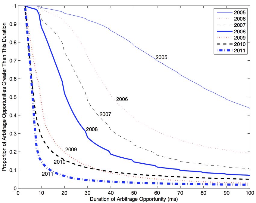
between the other three largest exchanges, NASDAQ, BATS and DirectEdge.17 Table 2 that correlations are higher when we treat the New York market as lagging Chicago than when we treat the Chicago market as lagging New York or treat the two markets equally. 99.99% of the arbitrage opportunities we identify are “good arbs,” meaning that deviations of the ES-SPY spread from our estimate of fair value that are large enough to trigger an arbitrage nearly always reverse within a modest amount of time. This is one indication that our method of computing the ES-SPY arbitrage opportunity is sensible. 5.2.3 Mechanical Arbitrage Over Time: 2005-2011 In this sub-section we explore how the ES-SPY arbitrage opportunity has evolved over time. Figure 5.3 explores the duration of ES-SPY arbitrage opportunities over the time of our data set, covering 2005-2011. As can be seen in Figure 5.3a, the median duration of arbitrage opportu- nities has declined dramatically over this time period, from a median of 97 ms in 2005 to a median of 7 ms in 2011. Figure 5.3b plots the distribution of arbitrage durations over time, asking what proportion of arbitrage opportunities last at least a certain amount of time, for each year in our data. The figure conveys how the speed race has steadily raised the bar for how fast one must be to capture arbitrage opportunities. For instance, in 2005 nearly all arbitrage opportunities lasted at least 10ms and most lasted at least 50ms, whereas by 2011 essentially none lasted 50ms and very few lasted even 10ms. Figure 5.4 explores the per-arbitrage profitability of ES-SPY arbitrage opportunities over the time of our data set. In contrast to arbitrage durations, arbitrage profits have remained remarkably constant over time. Figure 5.4a shows that the median profits per contract traded have remained steady at around 0.08 index points, with the exception of the 2008 financial crisis when they were a bit larger. Figure 5.4b shows that the distribution of profits has also remained relatively stable over time, again with the exception of the 2008 financial crisis where the right-tail of profit opportunities is noticeably larger. Figure 5.5 explores the frequency of ES-SPY arbitrage opportunities over the time of our data set. Unlike per-arb profitability, the frequency of arbitrage opportunities varies considerably over time. Figure 5.5a shows that the median arbitrage frequency seems to track the overall volatility of the market, with frequency especially high during the financial crisis in 2008, the Flash Crash on 5/6/2010, and the European crisis in summer 2011. This makes intuitive sense: when the market is more volatile, there are more arbitrage opportunities because there are more jumps in one market that leave prices temporarily stale in the other market. Figure 5.5b confirms this intuition formally. The figure plots the number of arbitrage opportunities on a given trading day against a measure we call distance traveled, defined as the sum of the absolute-value of changes in the ES midpoint price over the course of the trading day. This one variable explains nearly all of
18

        Figure 5.3: Duration of ES & SPY Arbitrage Opportunities Over Time: 2005-2011
Notes: Panel (a) shows the median duration of arbitrage opportunities between the E-mini S&P 500 future (ES)
and the SPDR S&P 500 ETF (SPY) from January 2005 to December 2011. Each point represents the median
duration of that day’s arbitrage opportunities. The discontinuity in the time series (5/30/2007-8/28/2007) arises
from omitted data resulting from data issues acknowledged by the NYSE. Panel (b) plots arbitrage duration against
the proportion of arbitrage opportunities lasting at least that duration, for each year in our dataset. Panel (b)
restricts attention to arbitrage opportunities with per-unit profits of at least 0.10 index points. We drop arbitrage
opportunities that last fewer than 4ms, which is the one-way speed-of-light travel time between New York and
Chicago. Prior to Nov 24, 2008, we drop arbitrage opportunities that last fewer than 9ms, which is the maximum
combined effect of the speed-of-light travel time and the rounding of the CME data to centiseconds. See Section
5.2.1 for further details regarding the ES-SPY arbitrage. See Section 4 for details regarding the data.

       (a) Median Arb Durations Over Time                          (b) Distribution of Arb Durations Over Time
19
Figure 5.4: Profitability of ES & SPY Arbitrage Opportunities Over Time: 2005-2011
Notes: Panel (a) shows the median profitability of arbitrage opportunities (per unit traded) between the E-mini
S&P 500 future (ES) and the SPDR S&P 500 ETF (SPY) from January 2005 to December 2011. Each point
represents the median profitability per unit traded of that day’s arbitrage opportunities. The discontinuity in the
time series (5/30/2007-8/28/2007) arises from omitted data resulting from data issues acknowledged by the NYSE.
Panel (b) plots the kernel density of per-arbitrage profits for each year in our dataset. See Section 5.2.1 for details
regarding the ES-SPY arbitrage. See Section 4 for details regarding the data.
(a) Median Per-Arb Profits Over Time (b) Distribution of Per-Arb Profits Over Time
the variation in the number of arbitrage opportunities per day: the R2 of the regression of daily
arbitrage frequency on daily distance traveled is 0.87.
Together, the results depicted in Figures 5.3, 5.4 and 5.5 suggest that the ES-SPY arbitrage
opportunity should be thought of more as a mechanical “constant” of the CLOB market design
than as a profit opportunity that is competed away over time. Competition has clearly reduced the
amount of time that arbitrage opportunities last (Figure 5.3), but the size of arbitrage opportuni-
ties has remained remarkably constant (Figure 5.4), and the frequency of arbitrage opportunities
seems to be driven mostly by market volatility (Figure 5.5). Figure 5.2 above, on the time series
of correlation breakdown, reinforces this story: competition has increased the speed with which
information from Chicago prices is incorporated into New York prices and vice versa (the analogue
of Figure 5.3), but competition has not fixed the root issue that correlations break down at high
enough frequency (the analogue of Figure 5.4).
These facts both inform and are explained by our model in Section 6.
5.3 Discussion
In this section, we make two remarks about the size of the prize in the speed race.You can also read