The Human Capital - Reproductive Capital Tradeoff in Marriage Market Matching
←
→
Page content transcription
If your browser does not render page correctly, please read the page content below
The Human Capital - Reproductive
         Capital Tradeoff in Marriage Market Matching
                                          Corinne Low∗
                                      September 3, 2021

    For much of recent history, the relationship between women’s human capital and
men’s income was non-monotonic: while college-educated women married richer spouses
than high school-educated women, graduate-educated women married poorer spouses
than college-educated women. This can be rationalized by a bi-dimensional matching
framework where women’s human capital is negatively correlated with another valuable
trait, fertility, or “reproductive capital.” I use a transferable utility matching model to
show that bi-dimensionality with negatively correlated traits can produce non-monotonicity
in income matching as a general feature. While the equilibrium match depends on the
distribution of female types, I provide a condition under which non-monotonicity will
always appear for any distribution of women with a sufficiently rich distribution of men.
A simulation of the model using Census fertility and income data shows that it can predict
the recent transition to more assortative matching as assisted reproduction technologies
have increased and desired family sizes have fallen.
    JEL Codes: J12, J13, J16, D13, C78

1       Introduction

It has long been suspected that higher earning may not always yield women wealthier
mates. Early theory on marriage markets predicted that in fact matching should be
negative assortative in incomes, due to returns to specialization [Becker, 1973]. Recent
research suggests that earning high income itself could make women less desirable to
    ∗
    Wharton Business Economics and Public Policy Department, corlow@wharton.upenn.edu. I am
indebted to Pierre-André Chiappori, Cristian Pop-Eleches, Bernard Salanié, Nava Ashraf, Gary Becker,
Alessandra Casella, Varanya Chaubey, Don Davis, Jonathan Dingel, Lena Edlund, Clayton Featherstone,
Claudia Goldin, Tal Gross, Joe Harrington, Murat Iyigun, Rob Jensen, Navin Kartik, Judd Kessler,
Ilyana Kuziemko, Jeanne Lafortune, Kathleen McGinn, Olivia Mitchell, Michael Mueller-Smith, David
Munroe, Suresh Naidu, Sonia Oreffice, Ernesto Reuben, Aloysius Siow, Kent Smetters, Sebastien Turban,
Miguel Urquiola, Eric Verhoogen, Alessandra Voena and many seminar participants for helpful comments
and advice. I thank the editor and three anonymous referees for their excellent suggestions, and Cung
Truong Hoang and Hira Abdul Ghani for excellent research assistance.

                                                  1
potential partners [Bursztyn et al., 2017, Bertrand et al., 2015]. And yet matching is
generally positive assortative on income, and most literature shows it has become more so
over time [Chiappori et al., 2017b, Hurder, 2013, Greenwood et al., 2016, 2014, Fernandez
et al., 2005, Schwartz and Mare, 2005].1
In this paper, I posit that underlying these apparent contradictions is the fact that hu-
man capital investments that yield greater income may also decrease another desirable mar-
riage market trait, “reproductive capital.” Women’s fertility decreases with age, and human
capital investments that increase income may delay marriage and childbearing and increase
spacing between births. I first show that older age at marriage is linked to lower spousal in-
come for women, even when controlling for own income, aligning with experimental findings
that men value women’s age, through the channel of fertility [Low, 2021]. I then document,
for the first time, that husband’s income has historically exhibited a non-monotonic pattern
in wife’s education: additional education up to a college degree was associated with increased
spousal income, but education beyond college was associated with decreased spousal income.
This pattern cannot be rationalized by a traditional unidimensional model, but can be easily
explained by a bi-dimensional model where income is negatively correlated with fertility.
I outline a transferable utility matching model between men characterized by income
and women characterized by income and fertility. A latent “human capital type” impacts
both income and fertility, with fertility weakly decreasing in income. I demonstrate that
with a surplus function that is supermodular in both incomes and income and fertility, and
no further restrictions, such a model can produce either positive or negative assortative
matching on income, depending on the distribution of types. Non-monotonic matching will
always be possible as long as some women differ in income only and not fertility, and other
women have higher income but sufficiently lower fertility. Finally, if the surplus function
features diminishing relative complementarity in incomes compared to that between income
and fertility, then for any distribution of female types there can always be non-assortative
matching as long as the richest man is “rich enough.”
This contributes to a growing literature showing that truly multidimensional models,
as opposed to index frameworks, may be crucial in understanding matching patterns,
1
Note that Gihleb and Lang [2016] and Eika et al. [2019] do not find increasing assortativeness over time.
2since valuations of of non-income traits likely vary with income [Chiappori et al., 2017a,
Galichon and Salanié, 2015, Coles and Francesconi, 2011, Lindenlaub and Postel-Vinay,
2017, Dupuy and Galichon, 2014, Galichon et al., 2019, Coles and Francesconi, 2019].
To further explore the implications of the model, I introduce a specific example surplus
function that would produce assortative matching in a unidimensional model, but can
produce non-monotonic matching in incomes due to the presence of reproductive capital.
I show that the equilibrium can change based either on the tradeoff between human and
reproductive capital in women’s type distribution, or shifts in men’s income distribution.
I then show that when education is made endogenous, the education decision will depend
on the matching penalty, aligning with theoretical and empirical work showing fertility
concerns can affect career investments [Siow, 1998, Dessy and Djebbari, 2010, Zhang, 2021,
Gershoni and Low, 2021b], but highlighting the equilibrium matching channel in addition
to personal utility loss from lower fertility. Nonetheless, I show it is possible to sustain
an equilibrium where women invest in human capital despite worse matching outcomes,
because they value the wage returns over the marriage market penalty.2
Finally, I simulate the model using Census data on income and fertility over time,
and demonstrate that it can match the evolution of historical patterns. The convergence
between highly educated and college educated women’s fertility rates as average family
sizes fell can produce the shift from non-monotonic to assortative mating, matching a
broader “reversal of fortune” for educated women on the marriage market [Fry, 2010, Rose,
2005, Isen and Stevenson, 2010, Bertrand et al., 2020]. Moreover, the model can match
the increases in women pursuing graduate education over time.
Together, these results demonstrate that while we may presume women value fertility
personally, it also affects them economically. This paper uses different levels of education
to demarcate human capital investments, standing in for the more general problem of the
tradeoff between career investments and fertility, which is of first-order concern to women.3
2
This contributes an example where investments can affect multiple dimensions to the literature on
premarital investments [Iyigun and Walsh, 2007, Peters and Siow, 2002, Lafortune, 2013, Dizdar, 2018,
Mailath et al., 2013, Cole et al., 2001, Nöldeke and Samuelson, 2015, Mailath et al., 2017].
3
For evidence that it is difficult to co-process career investments and fertility, see Goldin and Katz
[2002], Bailey [2006], Bailey et al. [2012], Adda et al. [2017], Kleven et al. [2019], and Gershoni and Low
[2021a] for evidence that future reproductive time horizons drive young women’s decision-making.
3Individuals, policymakers, and firms may be able to use a better understanding of this
tradeoff to blunt the impact of reproductive capital’s decline.
The remainder of the paper proceeds as follows: Section 2 documents stylized facts,
Section 3 develops a model that incorporates fertility in the marital surplus function,
Section 4 simulates the model, and Section 5 concludes.
2 Stylized Facts
In this section, I establish two new stylized facts. The first is that older age at first
marriage for women is associated with poorer spouses, even conditional on own income.
The second is that women’s human capital, which increase earnings but decrease fertility,
has historically been non-monotonically related to spousal income.
First, Figure 1 shows that for women over the age of around 25, each year older that
they marry is associated with lower spousal income.4 Although the negative relationship
between women’s age and spousal income is only correlational, the fact that individuals
who marry later tend to be positively selected makes it suggestive of a negative impact
of age on marriage market outcomes.5
Appendix Figure A1 conditions on income to show that in addition to the average
pattern, at each level of women’s own income, marrying older is linked to marrying a
poorer spouse for women (but not for men). This aligns with evidence from an incentive-
compatible experiment in Low [2021] that men have a negative preference for women’s
age when it is randomly assigned to dating profiles. The fact that it is driven by men
with accurate knowledge of the fertility-age tradeoff and who have no children themselves
suggests an underlying preference for fertility.
If men indeed value fertility as a marriage market trait, it suggests that time-consuming
human capital investments would be a double-edged sword for women: on the one hand,
4
This pattern is shown in women 46-55 at the time of the 2010 American Community Survey, so
that marriages up to age 45 can be shown. This pattern is consistent in younger ages and earlier years.
5
One might worry the pattern stems from unobservable selection, if women who marry later are
“leftover”. However, the pattern of marriage volume makes this unlikely, since the bulk of marriages—and
thus the largest possible sorting—occurs before the decline in husband’s income begins, as shown by
the density graph. Zhang [2021] additionally notes that the selection of men who marry late tends to
be negative, but we do not see the same declining spousal income for men.
4Figure 1: Spousal Income by Age at Marriage
Notes: Lines represent the average spousal income for first marriages by age at marriage for women versus men. Bars
represent the portion of all women’s marriages occurring at that age, to check whether selection is driving the effect. Source:
2010 American Community Survey (1 percent sample) marital histories for white men and women, 46-55 years old.
human capital carries higher earning, a presumably positive attribute likely to help attract
a high-income spouse. On the other hand, income-increasing investments take time, de-
creasing what could be another valuable asset on the marriage market, reproductive capital.
While much empirical work categorizes all women with college degrees as “college plus,”
the “reproductive capital” hypothesis suggests women with college degrees and graduate
degrees may have very different marriage market outcomes, since women with college
degrees only could still marry quite young and have large families. Moreover, graduate
degrees are correlated with the types of high-investment careers that may continue to
interfere with time to have children: the tenure track, the partner track, surgical residencies,
and climbing the corporate ladder, all investments typically made in one’s thirties.
Figure 2 shows that when graduate and college education are separated, historically,
there was a non-monotonic relationship between women’s education and men’s income. All
levels of education prior to a graduate degree are associated with higher income, whereas
graduate degrees are associated with lower spousal income, up until the 1990s.6
6
US Census and ACS 1% sample, restricted to women 41-50, so that the vast majority of first marriage
activity and educational investments have already taken place by the time they are observed.
5Figure 2: Non-monotonicity in spousal income by wife’s education level Notes: Income of spouse based on wife’s education level.
of the data, but not the apparent “penalty” to graduate education.
     Moreover, while literature has noted a general increase in marriage rates (and decrease
in divorce rates) for educated women, these changes were actually driven specifically by
graduate-educated women, as shown in Appendix Figure A2. College educated women
historically have, in fact, had comparable marriage and divorce rates to women with less
education. Only highly educated women previously married substantially less and divorced
more, until a recent improvement.
     A bi-dimensional model where a second factor decreases in education, even as income
rises, can help explain this data. As shown in Table 1, Census data shows a substantial
difference between college and highly educated women’s number of children in 1970, while
the difference between those with college degrees and those with high school education
or some college is substantially smaller, especially when it comes to the proportion with
greater than 4 children. Note that while highly educated women marry older than other
educational levels, the difference in fertility appears to stem from more than just this
difference, potentially reflecting differences in post-education career investments as well.

Table 1: Income, Spousal Income, Age at Marriage, and Children by Women’s Education

                                          ≤ High Some College Highly Highly Ed. -
                                          School College Ed.   Ed.   College Ed.
           Income                          10,179        14,220        18,879       32,986         14,107***
           Spousal Income                  43,205        64,247        79,147       73,621         -5,526***
           Age at marriage                  21.28         22.42        23.63         24.36          0.73***
           Children in HH                    2.51         2.56          2.63         2.19           -0.45***
           ≥ 4 children in HH                0.25         0.25          0.25         0.16           -0.09***
Notes: 1 percent 1970 Census data, women 41-50, except for children in household, which is measured for women 38-42, to
avoid bias from children aging out of the household, weighted by Census person weights. Children ever born is available in
1970, but not in 2000 or 2010, which is required for the simulations. Additionally, it may not reflect true fertility, since in
earlier years it may have been more common for children to die in infancy. Nonetheless, the gap between College and Highly
Educated women for this metric is extremely similar: 0.42 fewer children born, and a 0.11 lower chance of having ≥4 children.

     Thus, in the next section I develop a model of matching where human capital invest-
ments increase income, but decrease fertility. While other elements in addition to fertility
could be negatively correlated with income, they may be less likely to be complementary

                                                              7
with income, which is a key driver of the model’s ability to produce non-monotonic income
matching patterns.7 I explore some of these alternative explanations in Appendix C.4, and
also discuss generalizing the model’s insights to other settings in Section 3.1.3. However,
even if the second factor is something other than fertility, the key point of the model and
empirical evidence introduced here is that the data appears to reflect a duality of human
capital investments for women that does not exist for men.
3 A Theory of the Marriage Market with Reproductive Capital
If men value women’s fertility, it will have consequences for matching patterns, as well
as women’s willingness to invest in human capital. This section studies these effects
using a bi-dimensional, transferable utility matching model. In this model, human capital
investments yield earnings gains, but can also delay marriage and childbearing, resulting
in lower fertility. The dimensions of this model cannot be collapsed to an index, because
fertility impacts the household’s ability to create surplus through investing income in
children, and thus its value is dependent on income.
Transferable utility matching models derive matching patterns from the efficient cre-
ation and division of surplus [Shapley and Shubik, 1971, Becker, 1973]. The equilibrium
payoff of each individual is set in the market as “offers” where both spouses are able to
attract one another. Thus, the model simply requires assumptions on the form of the
marital surplus to establish equilibrium matching patterns and resulting utilities. As long
as the assumptions are met for fully transferable utility, the disaggregate equilibrium will
be one and the same with the equilibrium that maximizes total social surplus.
3.1 General Model
This section demonstrates that a simple bi-dimensional model where couples care about
income and fertility can produce non-monotonic matching in incomes. In particular, match-
ing will always be assortative when women’s income varies, but fertility stays constant,
7
One thing that would likely function similarly is tastes for fertility. Thus, I cannot rule out that highly ed-
ucated women have lower tastes for children, rather than lower ability to have children. First, I consider this
similar to a reproductive capital argument, since, ultimately, it implies a male valuation of fertility. Secondly,
suggestive evidence in Appendix C.4 shows that selection may not be entirely the cause, since the spousal
income penalty moves little during a time when the number of women seeking graduate degrees doubled.
8but need not be when income and fertility vary in tandem.
3.1.1 Model Setup
There is a two sided market with a unidimensional side, “men,” and a bi-dimensional side,
“women.” Men are characterized solely by income, y ∈[0,Y ], and women are characterized
by both income and fertility, (z, p)∈[0,Z]×[0,1].8
Individuals care about both children and private consumption, with utility meeting
the generalized quasi-linear (GQL) form, which is the necessary and sufficient condition
for transferable utility [Bergstrom and Cornes, 1983, Chiappori and Gugl, 2014]. Thus,
through maximizing the sum of utility we can identify the household surplus function,
s(y, z, p), increasing in all arguments.
Let the surplus exhibit:
∂s2
• Supermodularity in incomes: ∂y∂z
>0
∂s2
• Supermodularity between men’s income and fertility: ∂y∂p
>0
3.1.2 Matching Equilibrium
This surplus function will always produce assortative matching in incomes when fertility
is equal across women.
Proposition 1. Let there be two men, y and y0, with y < y0. For any two women with
incomes z and z0, z0 > z, and fertility p, the stable matching matches y0 with (z0, p) and
y with (z, p).
Proof. With transferable utility, the stable match will maximize total surplus. Thus,
8
Although making men unidimensional is a simplification, it should be noted that other matching
models that feature multiple characteristics are actually unidimensional as long as the characteristics
can be collapsed to a single index. I focus on income as that is the key factor usually examined in models
looking at societal trends in assortative matching. Many of the predictions here would also hold for other
factors that could be part of a quality index, such as height or attractiveness.
9supposing by contradiction that y is paired with z0 and y0 with z, it must be that:
s(y, z0, p)+s(y0, z, p)>s(y0, z0, p)+s(y, z, p)
s(y, z0, p)−s(y, z, p))>s(y0, z0, p)−s(y0, z, p)
∂s(y, z, p) 0 , z, p)
Which would imply that, for a small change in z, ∂z
> ∂s(y ∂z , which would mean
s is submodular, contradicting the premise.
However, when fertility differs, the matching can be positive assortative or negative
assortative on incomes, depending on the income-fertility tradeoff for women.
Proposition 2. Let there be two women (z, p) and (z0, p0) with z p0. Let =z0 −z
and η = p−p0, both positive. Let λ = η . There exists a λ such that the stable matching
matches y with (z, p) and y0 with (z0, p0), and a smaller λ such that the stable matching
matches y with (z0, p0) and y0 with (z, p).
Proof in Appendix section B.1. Its intuition is that the stable match must maximize
surplus, and because the surplus is supermodular between both men’s income and women’s
income and fertility, it is always possible for the supermodularity in income-fertility to
“outweigh” that in incomes for a sufficiently high quantity of income relative to fertility. In
other words, the form of the stable match depends on the distribution of women’s traits.
These two propositions together imply non-monotonic matching is possible when some
women differ only in income, while others differ in income and fertility.
Lemma 1. Let z(y) represent the income of the woman matched with man of income y.
In a distribution where men vary in income, and women vary in both income and fertility,
where fertility is always weakly decreasing in income, it is possible for there to be two men
with incomes y and y0 > y such that z(y0) > z(y), and a third man with income y00 > y0
where z(y00)we can guarantee that there will always be a man rich enough such that he matches
non-assortatively in the stable match.
∂ 2 s(y,z,p)
∂y∂z
Lemma 2. For s(y, z, p) such that limy→∞ ∂ 2 s(y,z,p)
=0 , for any λ there exists a Y large
∂y∂p
enough that the stable match does not match him with the highest-income woman.
Proof. Assume by contradiction assortative matching everywhere. Then the richest man
Y is matched with the richest woman, with income and fertility (z0, p0). Define man ȳ that
is below Y and matched with woman with income and fertility (z̄, p̄), where z0 >z̄ and
p0 s(Y, z̄, p̄)+s(ȳ, z0, p0). Rearranging,
the left-hand side becomes s(ȳ, z̄, p̄)−s(ȳ, z0, p0)−(s(Y, z̄, p̄)−s(Y, z0, p0)), which has
the same sign (see Appendix B.1 for details) as:
Y
∂ 2s(θ, z, p) ∂ 2s(θ, z, p)
Z
λ − η dθ.
ȳ ∂θ∂z ∂θ∂p
∂ 2 s(y,z,p)
∂y∂z
For Y high enough, this will always be negative, since λ is fixed and ∂ 2 s(y,z,p)
is positive
∂y∂p
and goes to zero as y increases. Thus the richest man cannot be matched with the richest
woman for Y high enough.
Thus, a matching model that is unidimensional on one side and bi-dimensional on the
other can easily match empirical patterns exhibiting non-monotonicty along the “main” trait.
In fact, non-monotonicity will be a general feature of the model when the women’s traits are
negatively correlated and the top of the male income distribution is sufficiently high. Such
bi-dimensional matching frameworks may provide a way to reconcile the general tendency
toward assortative matching with deviations that appear to suggest some people do not value
income. Rather, it is likely that income is negatively correlated with another valuable trait.
3.1.3 Generalizing to Other Settings
While this model is described in terms of income and fertility, its insights can be generalized
more broadly. First, in terms of marriage market matching, one can think about insights
for any situation in which one side has two salient traits that are negatively correlated and
11whose contribution to the surplus increases in the other side’s quality. This is in contrast to
other useful work on bidimensional marriage models, such as Coles and Francesconi [2019],
where the value of partner income is decreasing in own income. The key insight of this
work is that even with supermodularity in incomes, it is possible to have non-assortative
matching depending on the underlying distribution of traits and the change in relative
complementarities across the income distribution. This provides predictions in line with
the empirical regularity of largely positive assortative matching on income.
The model’s insights can also be applicable to settings outside of fertility where one
side of the market is bi-dimensional, and the value of both traits is increasing in the other
side’s characteristics. For example, manufacturers defined by quality and matching with
upstream suppliers may care about both quality and speed. If these supplier traits are
negatively correlated, non-monotonic matching in qualities is possible depending on the
distribution of types. If furthermore the complementarity between qualities relative to
the complementarity between quality and speed is decreasing in own quality, the model
produces the result that for any distribution of quality and speed among the suppliers, a
sufficiently high quality manufacturer will not be matched with the highest quality supplier.
This type of model may help explain non-assortative matching in a variety of markets
where one expects supermodularity in the most salient trait.
3.2 Parameterized model
In order to further explore and illustrate the model’s implications, this section presents
an explicit surplus function that can be parameterized. Because we know that matching
is generally assortative on income, the model uses as its foundation a surplus function
that would yield assortative matching in a unidimensional setting. Introducing the second
dimension of fertility leads to a prediction of potentially non-monotonic matching.
3.2.1 Household Problem
Men are characterized by income, y, and women are characterized by both income, z, and
fertility, p. Individuals value private consumption, q, and children as a public good, Q,
which are complementary, producing the underlying force toward assortative matching
12[Lam, 1988] .9 With a single public and private good, the necessary and sufficient condition
for transferable utility is generalized quasi-linear (GQL) utility [Bergstrom and Cornes,
1983, Chiappori and Gugl, 2014]. The simplest form of GQL is Cobb-Douglas utility, or
“qQ” utility [Chiappori, 2017, Chiappori et al., 2017b], which I modify as q(Q+1) so that the
couple cares about private consumption even if children do not occur. The utilities are thus:
um =qm(Q+1)
uw =qw (Q+1).
The impact of biological fecundity is captured by only allowing households to invest in
Q if a child is born, with probability p.
Because utility is fully transferable with these utilities, the allocation of income between
children and private consumption can be found by maximizing the sum of utilities subject
to the budget constraint. Assuming they have children, the couple’s problem is thus:
max q(Q+1)
q,Q
s.t. q+Q=y+z.
Accordingly, the utility maximizing level of Q and the sum of private consumptions, q, is
given by:
y+z+1
q∗ = ,
2
y+z−1
Q∗ = .
2
If children were born with certainty, this would result in a very standard surplus function
that is supermodular in incomes, and would thus predict assortative mating on the marriage
0 0
market. However, households are constrained to Q = 0 and q = y + z in the case no
children realize, with probability p. Thus, joint expected utility from marriage, T , is a
9
This can be thought of as the human tendency to want children to have similar levels of consumption
as parents, a driving force in quantity-quality tradeoff models.
13weighted average between the optimal joint utility if a child is born and the constrained
utility from allocating all income to private consumption:
(y+z+1)2
T (y,z,p)=p +(1−p)(y+z).
4
If individuals remain single, they simply consume their incomes, and so the surplus
2
from marriage, is s(y,z,p)=p (y+z+1)
4
+(1−p)(y+z)−y−z, yielding the household surplus
function:
1
s(y,z,p)= p(y+z−1)2. (1)
4
The household surplus function in (1) is supermodular in incomes, and is also super-
modular in income and fertility. Thus, the stable match will depend on the distribution of
types, as shown Proposition 2. However, this surplus function meets the additional criteria
∂ 2 s(y,z,p)
∂y∂z
in Lemma 1 that lim 2 =0: the complementarity between incomes relative to the
y→∞ ∂ s(y,z,p)
∂y∂p
complementarity between income and fertility goes to zero as men’s income goes to infinity.
The intuition for this is that there is substitution between spousal incomes in generating
the household surplus, but not between husband’s income and wife’s fertility, and thus the
marginal tradeoff between fertility and wife’s income worsens as household income rises.
For simplicity, this example uses a binary fertility outcome, but the model is easily
extendable to a case with a set of possible family sizes, and a probability of achieving each
one, while maintaining the same properties, as shown in Appendix B.4. This multiple
children extension is the one I will use for simulations.
3.2.2 Distribution of Types
Women are divided into three types: low income and high fertility, L, medium income and
high fertility, M, and finally high income and low fertility, H. This captures a key feature
of biological fecundity, that it declines non-linearly past a certain age. As a result, some
amount of human capital can be acquired without incurring reproductive capital losses,
but larger human capital investments incur a reproductive capital penalty.10
10
There may be other costs to education, in terms of foregone time or monetary costs. However, for
this initial section, the education distribution is assumed to be exogenous. Additionally, it is possible
14Appendix D shows that a model with continuous female skill produces highly similar
predictions for aggregate matching patterns. Thus illustrating with three types does not
limit the model’s generality, but has the advantage of mapping well onto empirical exercises,
where education is typically used as women’s “type,” since income is chosen endogenously
post-marriage. Roughly, you can think of the three types as being high school, college,
and graduate-educated women.
The three types of women have the following income–fertility pairs:
z p
L: γ−µγ π+δπ
M: γ π+δπ
H: γ+δγ π
Thus, δγ is the income premium to being the high versus medium type, and δπ is the fertility
penalty. µγ is the income premium to being the medium versus low type. The mass of the
three types of women is first assumed to be exogenously given, as gK , where K ∈L, M, H.
Section 3.4 extends the model to allow for endogenous human capital investment.
There is a total measure 1 of women: gL +gM +gH =1. I assume there are more men
than women, and thus only measure 1 of men can be matched.11 Define the poorest man
who receives a match as y0 and the richest man as Y . Assume the income parameters are
such that the poorest matched man’s income plus the poorest woman’s income is greater
than 1 (this ensures interior solutions for the amount invested in children).
3.3 Matching Equilibrium
A matching is defined as the probabilities over the distribution of y types for matching
with each (z, p) type, and value functions u(y) and v(z, p) such that for each matched
pair u(y)+v(z,p)=s(y,z,p). That is, their individual surplus shares add up to the joint
that men make human capital investments as well, but these impact them uni-dimensionally.
11
This is for simplicity in pinning down explicit utilities. There could also be excess L-type women.
15surplus created by a match. A matching is stable if two conditions hold for all individuals:
u(y)+v(z,p)≥s(y,z,p)
u(y)≥y, v(z,p)≥z
That is, the utility received by any two individuals in their current matches must be jointly
higher than the surplus they could create by matching together (the equation holds with
equality if the pair is married to each other), and all individuals receive a positive benefit
to marriage versus the outside option of consuming their own income.
In this way, the surplus shares can be thought of as prices that clear the market for
marriage partners. Any stable match must maximize the aggregate marital surplus over
all possible assignments [Shapley and Shubik, 1971].
General traits of equilibrium The principle of surplus maximization allows us to
think about the stable equilibrium in terms of the relative benefit men of different incomes
receive from switching between types. That is, the stable match will be determined by how
the surplus benefit from switching types changes in men’s income. The surplus benefits
from changing types as a function of men’s income are as follows. Medium versus low:
∆M−L(y)=s(y,γ,π+δπ )−s(y,γ−µγ ,π+δπ )
1
= (π+δπ )µγ (2y+2γ−µγ −2).
4
High versus medium:
∆H−M (y)=s(y,γ+δγ ,π)−s(y,γ,π+δπ )
1 1
= πδγ (2y+2γ+δγ −2)− δπ (y+γ−1)2.
4 4
High versus low:
∆H−L(y)=∆H−M (y)+∆M−L(y).
∆M−L(y) is linear, and monotonically increasing in men’s income. Thus, there is always
16a higher surplus benefit from pairing a higher income man with a higher-income-type
woman, corresponding to the supermodularity in the surplus function. Thus, any stable
match must match M women with higher income men than L women.
∆H−M is quadratic, giving it a unique maximum. The implication of this is that there
is a single interval of men that it is maximally beneficial to pair with high-income women.
However, this interval may not be the richest men. Note that even when ∆H−M (y) is positive
over the full range of y, indicating that all men prefer H women to M women, the richest
men may not be matched with the richest women, because they do not value the match
sufficiently to pay the “price” these women command. This quadratic form stems from
the declining relative complementarity between incomes compared to income and fertility.
∆H−L(y) is also quadratic, implying that there is a unique interval of men that should
be matched with H versus L women, when relevant.
From this we can derive the following lemma.
Lemma 3. Any stable matching will exhibit the following three characteristics:
1. All matched men will be higher income than all unmatched men.
2. All men matched with M women must be higher income than all men matched with
L women.
3. The set of men matched with H women must be connected.
Proof. Item (1) follows from the fact that the surplus function is monotonically increasing
in men’s income (as long as the total household income exceeds 1, which was assumed).
Item (2) follows from the fact that the benefit to matching with an M type versus an L
type is monotonically increasing in income. Item (3) follows from the fact that the benefit
of matching with an H type versus M or L type is single-peaked: If there is a gap in the
men who are matched with H women, then the men in the gap must be matched with
L or M women. But, as the benefit to matching with H women over L or M women is
single-peaked, it cannot simultaneously be better to be matched with H women on both
sides of the gap than in the gap.
17Figure 3: Possible matches: H women match with...
(1) Top (2) Interior, top (3) Middle (4) Interior, bottom (5) Bottom
Y Y
Men’s income
y4 y3 y3 y3
y2 y2 y2 y1
y0 y0
L M H L M H L M H L M H L M H
Women’s type
The options for the match that meet these criteria are illustrated in Figure 3, where the
x-axis represents women’s type and the y-axis represents men’s income. The first picture
illustrates standard assortative matching. All other possible match types meet the criteria
in Lemma 3, and yet feature non-monotonicity in income-matching. Over some segment
of men, women’s income is increasing in men’s income. Over another, it is decreasing.
Full equilibrium characterization Type H women will be matched with the men
who receive the most benefit from matching with them relative to type M or L women.
Thus, we can think of characterizing the stable equilibrium as sliding a segment of length
h of men who match with type H women from the poorest man to the richest, stopping
where the total surplus is maximized. If the man at the top of this segment benefits more
than the man at the bottom, we should slide it up. If the man on the bottom benefits
more than the man at the top, we should slide it down.
Thus, assortative matching will only be stable when the man with income Y receives
more benefit to an H match than the poorest man to be matched with an H type, labeled
as y4 in Figure 3.12 This leads to the following proposition:
Proposition 3. Let Y represent the income of the richest man. For any set of parameters,
it is possible to find a Y large enough such that the equilibrium match is non-monotonic
in income.
Proof. Assortative matching requires that ∆H−M (Y ) ≥ ∆H−M (y4), because otherwise
the total surplus can be increased by matching the man right below y4 with an H type
12
Note that these thresholds have specific definitions in terms of the distributions, but I name them
for notational simplicity. y4 =F −1(1−gH ), y3 =F −1(1−gM ), y2 =F −1(gL), and y1 =F −1(gH ).
18woman, and Y with an M type woman. Plugging in the surplus differences, the condition
π
becomes: δ ≥ 12 (Y
δπ γ
+y4)+γ−1, which relies linearly on Y . Assume this condition is met.
Increasing Y sufficiently will cause the condition to be violated, in which case matching
Y with an H-type woman cannot be surplus maximizing.
We can envision moving through each of the equilibria by slowly increasing Y relative
to the other parameters. When the condition for assortative mating fails, H-type women
match interior to the segment of men matching with M-type women, as shown in equilib-
rium 2, such that the benefit of the bottom man matching with an H-type with income y∗
is exactly equal to the income of the top man with income y∗∗:13 ∆H−M (y∗)=∆H−M (y∗∗).
As Y increases, this segment will continue sliding down until there are no more M women.
At that point, to slide it down further requires comparing the benefit to matching with
an L type woman versus an H type woman. Thus, equilibrium 3, where H women are
matched exactly between L and M women, will be stable as long as the last man matched
with an M woman, with income y3, receives less benefit from an H versus M match than
the last man matched with an L woman, labeled y2, but receives more benefit from an
H versus L match. When man y3 receives less benefit from an H versus L match than
y2, the segment slides interior to the men matching with L-type women, as in equilibrium
4, such that ∆H−L(y∗)=∆H−L(y∗∗). Finally, if Y continues to increase, at some point the
lowest income man, y0, will be matched with an H type woman, as in equilibrium 5.
Proposition 4. The unique stable match is fully characterized by Lemma 1 and the
following conditions:
• If ∆H−L(y1)≤∆H−L(y0),
H women match with poorest men, from y0 to y1.
• If ∆H−L(y3)∆H−L(y0),
H women match with men interior to the set matching with L women, where
∆H−L(y∗)=∆H−L(y∗ +h).
¯ ¯
13
where y∗∗ =F −1(F (y∗)+gH ).
19• If ∆H−L(y3)≥∆H−L(y2) and ∆H−M (y3)≤∆H−M (y2),
H women match with middle men, from y2 to y3.
• If ∆H−M (Y )∆H−M (y2),
H women match with men interior to the set matching with M women, where
∆H−M (y∗)=∆H−M (y∗ +h).
¯ ¯
• If ∆H−M (Y )≥∆H−M (y4),
H women match with richest men, from y4 to Y .
Proof. The conditions in Lemma 1 create a single-variable maximization problem that has
a unique solution for any given parameters, as shown in Appendix B.2. The solution is
found through the first-order conditions of the problem, and the cutoffs for each equilibrium
type is found through the boundaries for corner solutions.
Figure 4: Illustration of surplus difference conditions for each matching equilibria
(1) Top (richest) (2) Interior, top (3) Middle
∆ ∆ ∆
∆H−L ∆H−L < ∆H−L
< = >
∆H−M ∆H−M ∆H−M
L M H L H L H M
y y y
y0 y4 Y y0 y∗ Y y0 y2 y3 Y
(4) Interior, bottom (5) Bottom
∆ = ∆ >
∆H−L ∆H−L
∆H−M ∆H−M
H M H L M
y y
y0 y∗ Y y0 y1 Y
These conditions are illustrated in Figure 4. Note that although this figure illustrates
the changing equilibria by keeping other parameters fixed and moving the range of y, it is
20also possible to keep men’s distribution fixed and move the distribution of women’s types,
through changing the human capital return to investment or its fertility penalty, as is likely
with technological change. Appendix Figure A3 shows the range of δγ , the financial return
to investment, and δπ , the fertility penalty, that support different equilibria types. As δγ /δπ
increases, the matching progresses from equilibrium 5 to equilibrium 1, assortative matching.
Utility Transferable utility matching models allow the direct calculation of each individ-
ual’s equilibrium utility (value function). This is done through using the equilibrium stability
condition that u(y)+v(z,p)≥s(y,z,p), and that marriages improve welfare over singlehood.
This procedure is shown in Appendix B.3. Let women’s value functions for each type be
denoted U K , and the marital surplus each type receives as vK , constants that depend on the
underlying parameters, including δπ . Then women’s equilibrium utility for each type will be:
U H =γ+δγ +vH ,
U M =γ+vM ,
U L =γ−δµ +vL.
Note that individuals maximize the surplus they receive, rather than the “quality” of
their partner. So, from the woman’s perspective, a non-assortative equilibrium can be
viewed as women choosing relationships in which they have more “bargaining power,” thus
receiving a larger share of a slightly smaller pie. They can command this higher surplus
share when they create more relative value in relationships with lower earning partners.
However, the H-type equilibrium utility function is affected by the fertility loss asso-
ciated with education, both through her own lower utility from children, and through the
equilibrium channel of a smaller marital surplus share. If she only cared about fertility,
and her partner did not, her utility loss from the fertility costs of education would be
considerably reduced.
213.4 Endogenous Human Capital Investment
Both the personal and marriage market impacts of human capital investment will influence
women’s willingness to invest in human capital in the first place. The reproductive capital
loss creates an extra “tax” on women’s human capital investments, reducing the returns to
intensive human capital investments. However, it is still possible to sustain an equilibrium
where women invest in costly human capital, even if in doing so they forego the most
favorable marriage market matches.
Assume that the distribution of L types is fixed, but that M types can invest to
become H types. Further assume that women considering investing face a utility cost, ci,
of investment.14 Using the equilibrium value functions, women will invest in becoming the
high type when:
ci ≤U H −U M
ci ≤vH −vM +δγ
The mass of H types will now be endogenously determined as a function of the under-
lying density of ci. This mass affects the marital surpluses for each female type through
its impact on the y at the boundary between different wife types. Thus, the cutoffs for
women investing can be solved for as a fixed point of ci = vH (ci)−vM (ci)+δγ . Call the
solution to this equation ĉ. There will be a unique equilibrium where all women with costs
below ĉ invest in becoming the H type, and then match according to Proposition 1. If
no women invest, the matching will be assortative between L and M types. The threshold
cost for investment ĉ is decreasing in δπ (fewer women invest as the fertility cost rises) and
increasing in δγ (more women invest as the income premium rises).
Figure 5 illustrates the portion of women that invest and resulting matching equilibria
for different income gains and fertility costs of investments, and a heterogenous uniform
utility cost.15 Importantly, some women invest in all possible marriage market equilibria,
14
Including men’s human capital investments as well would complicate the model, as there could
potentially be multiple equilibria. However, in this model, men would not necessarily be expected to invest
more in response to women’s investments, since women’s investments also decrease reproductive capital.
15
The thresholds for the matching equilibria are somewhat different than in Appendix Figure A3, as
22except when H-type women are matched with the absolute lowest income men.
Figure 5: Matching Equilibrium and Investment by Income Return and Fertility Penalty
Notes: Bounds calculated with men’s income uniform from 0 to 6, and for women M-type income of 4, L-type income of 2,
with a mass of 0.35 L types, and 0.65 M types who have the option to invest. Baseline fertility is 0.3. Cost of investment
ranges uniformly from 0 to 12.
The figure illustrates the interesting difference in the forces driving women’s investment
decision versus the marriage market equilibrium. Women’s investment changes more in
δγ , the financial return to investment, while the marriage market equilibrium is more
influenced by δπ the fertility penalty. This is because women get the direct financial benefit
of their investment in addition to the marriage market payoff, and thus receive an extra
financial incentive to invest that does not appear in the marital surplus, which is what
influences the matching equilibrium. Thus, women may still be better off investing than
not, and yet experience a lower match quality.
3.5 Empirical predictions
Non-monotonic matching The first empirical prediction of the model is that the
matching relationship between men’s and women’s income can be non-monotonic. If
the equilibrium responds endogenously to the number of educated women on the market.
23income and fertility are negatively related in the distribution of women, the richest men
will not be matched with the richest women as long as either the fertility-income tradeoff
is large enough or the income of the richest man is high enough. This prediction matches
the stylized facts shown in Section 2.
Trend toward assortativeness and higher investment The model predicts that
if either δπ , the fertility penalty to investment, falls, or δγ , the income premium, rises,
matching will become more assortative at the top of the female income distribution, and
women will invest more in human capital. An increase in δγ is natural to think about, as
women may experience less discrimination in high-earning professions, and the returns to
skill on the labor market are rising. δπ is also likely to be rising over time, making the
time impact of women’s investments less costly from a reproductive perspective, both due
to improved technology and falling desired family sizes.
The model could also be extended to predict higher marriage and lower divorce rates
for highly educated women over time, by using a stochastic joint shock that makes some
couples choose not to marry, and others to divorce. Higher surplus couples would be more
resilient to higher shocks, and so marriage would be proportional to the surplus of the
couple, and thus when highly educated women match with poorer men, we would expect
lower marriage and higher divorce rates for this group than when they match with richer
men.16 These predictions are both explored in the following section.
4 Model Simulation Compared to Historical Data
In this section, I demonstrate the relevance of a bi-dimensional model with “reproductive
capital” to historical data by simulating the model with moments from Census data, and
demonstrating it can match shifts in matching patterns and marriage rates over time.
Simulating the model when people actually have multiple children requires introducing
a slightly more complex structure than a single fertility probability. Instead of constraining
16
One could also get a similar prediction with individual shocks. Recall that an H-type woman’s total
utility if married is U H =γ+δγ +vH . The “marital premium,” vH , is a function of both δγ and δπ . If she
is unmarried, she is unaffected by δπ . So, as fertility technology improves or desired family size falls, the
marital premium for H-type women increases, which would be tied to increased marriage and decreased
divorce rates.
24investments in children to be zero with probability p, I use an education-specific probability
of achieving each family size, and constrain investments in children proportionally based
on realized family size, as follows:
4
X c y+z+1 c y+z−1
s(y, z, p)= pc y+z− −y−z (2)
c=0
4 2 4 2
See Appendix B.4 for details on how this surplus is produced from underlying utilities.
4.1 Data Moments
Two key pieces of data from the decadal Census are used to feed the simulation. First,
incomes of men and women conditional on education. And, second, an education-specific
fertility distribution. For income, men’s income is drawn unconditional on education, and
then a net present value is calculated to approximate lifetime earnings. The patterns
shown are not sensitive to the exact method of approximation. Women’s income is drawn
conditional on educational level, for women working full-time, who stand in for the earning
potential of an individual at a given education level, since couples may decide to reallocate
a woman’s human capital toward home production. Details are provided in Appendix C.1.
For fertility, I use the empirical distribution of number of children conditional on
education. As shown in Figure 6, in 1970 highly educated women had substantially fewer
children and a higher probability of having zero children than college educated women.17
While highly educated women do marry approximately one year older than college educated
women on average, this difference likely also stems from longer child spacing and a higher
opportunity cost of maternity leave. Thus, I take the overall lower fertility as the best
measure of the tradeoff in reproductive capital from achieving higher income.
These moments change over time, which will drive changes in matching patterns in
the model. Market opportunities for women have naturally risen dramatically in the past
50 years [Hsieh et al., 2019]. However, a more dramatic shift might come from changes
in the fertility penalty associated with investment. One reason is changing technology,
17
And note, college educated women do not have a lower chance of having children than those with
lower education levels.
25Figure 6: Empirical Distribution of Children by Education Level and Year
Notes: Children currently at home for women 38-42 years old. Children ever born, only available through 1990, produces
qualitatively similar results, in Appendix Figure A4. “Highly educated” constitutes all graduate degrees. Source: 1 percent
Census data from 1970 and American Community Survey from 2010, weighted by person weights.
including fertility drugs, in vitro fertilization, surrogacy, egg donation, and egg freezing
(see, for example, Gershoni and Low [2021a,b]). Additionally, an overall trend toward
smaller family sizes [Doepke and Tertilt, 2009, Gould et al., 2008, Isen and Stevenson,
2010, Preston and Hartnett, 2010] causes highly educated women’s fertility to be more
comparable to college educated women’s fertility, as shown in the right side of Figure 6,
where college and graduate-educated women have a nearly identical fertility distribution
by 2010. This change could be driven by an increasing preference for child quality over
child quantity, which tends to accompany economic development [Becker et al., 1990].18
18
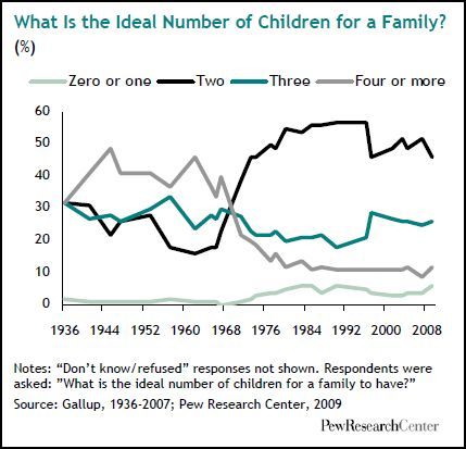
Not only did actual family sizes fall, but desired family sizes have fallen substantially. During the
1970s, there was a rapid transition from “four or more” as the modal answer for ideal family size to “two,”
shown in Appendix Figure A5 [Livingston et al., 2010].
26Figure 7: Spousal Income by Education Group
(a) Data (b) Simulation
Notes: Left-hand side figure comes from 1% Census data from 1960, 1970, 1980, and 1990, and American Community Survey
from 2000 and 2010, women 41-50 years old, weighted by Census person weights. Right-hand side is model simulation taking
random weighted draws of income (conditional on education for women), and then calculating an NPV of approximate
lifetime income conditional. Fertility distribution is for women 38-42, so children are still at home. Income is translated into
an NPV of 25 periods for men and 20 for women (robust to other choices). Using these inputs, matches are determined to
maximize total surplus, and then average income of predicted spouse is graphed by education group.
4.2 Simulation Compared to Data
Figure 7 shows on the left-hand side the changes in spousal income for women of differ-
ent education levels over time. The right-hand side simulates these same changes using
hypothetical spouses from matching according to surplus maximization of the function
in equation 2, plugging in the changes in the income distribution of men and women and
the empirical distribution of children over time.
Using only changes in income and fertility over time, the simulation captures the
crossing between the spousal incomes of college-educated and graduate-educated women,
matching the timing between the 1990 and 2000 Censuses. The matching patterns be-
tween other groups remain stable in the simulation, as they do in the data. While the
simulation somewhat over-estimates the differences between groups, as individuals are
assumed to match on income and fertility only, it demonstrates that even a very simple
model incorporating fertility can explain the non-monotonic relationship between spousal
income and women’s education, and later return to monotonicity.
Figure 8 compares the actual path of women’s investment in graduate education to that
predicted by the model. The distribution of the cost of education, ci, is calibrated to match
27Figure 8: Predicted Education
Notes: Model simulation of endogenous education decision, with uniform education cost, taking
NPV of approximate lifetime income conditional on education and fertility as inputs. Matching
and education decisions are determined to maximize surplus, as the private education decision will
match the efficient equilibrium.
the rates of graduation in 1970. Using that same cost distribution, the model matches the in-
crease in 1980 and 1990, although slightly overestimates the increase in 2000 and 2010. Note,
the distribution of ci used in the simulation is uniform–a cost distribution with lighter tails
may do a better job matching changes in later years. Nonetheless, this demonstrates that
even a simulation of the model without extensive calibration can rationalize historical facts.
When the spousal matching patterns are re-estimated using endogenous education
decisions, matching patterns are similar, although it exaggerates the difference between
highly and college educated women’s spousal income in later years because of the additional
selection effect, shown in Appendix Figure A6.
The model can also produce a simulation of marriage rates that matches the increasing
rates of marriage for highly educated women relative to college educated women over time,
shown in Appendix Figure A7.
This exercise demonstrates that a model where women’s reproductive and human
capital both matter in matching can reconcile historical patterns in women’s education
decisions and marriage market outcomes. The model’s bi-dimensionality is key to its
28success in matching the increasing spousal income at most levels of education—those that
do not carry significant fertility penalties—and decreasing spousal income, until recently,
between college and graduate education.
5 Conclusion
This paper treats women’s decisions as a tradeoff between two assets: human capital,
which grows based on investment, and reproductive capital, which depreciates with time. I
develop a bi-dimensional marriage matching model where women’s career investments affect
both human and reproductive capital. Matching is predicted to be non-monotonic when
the fertility cost of career investments are large relative to the income gains. This adds
a second cost to women considering time-consuming career investments—not only do they
themselves potentially lose out on fertility, but they experience a “tax” on the marriage
market as well. I document in US Census data that until recently marriage matching
followed the non-monotonic pattern predicted by the model. As family size desires fell and
reproductive technology expanded, equalizing family sizes between college and graduate
educated women, there has been a transition to more assortative mating, higher rates of
graduate education, and higher marriage and lower divorce rates for graduate educated
women. These patterns are matched by a simulation of the model.
This paper provides an example where a bi-dimensional matching framework is crucial
to rationalizing surprising patterns in the data. Moreover, it explores the occurrence of
non-monotonicty in income matching as a potentially general feature of such bi-dimensional
models where one side’s traits are negatively correlated.
This paper shows that reproductive capital is an important consideration in under-
standing both marriage patterns and women’s human capital decisions, showing how the
fertility costs of human capital investments may affect women economically, even if they
themselves do not desire children. More broadly, the concept of reproductive capital
suggests substantial welfare costs of aging for women, or secondary infertility caused by
poor medical care in developing countries.
29You can also read