Time series analysis in astronomy - Simon Vaughan University of Leicester

Time series analysis
   in astronomy

    Simon Vaughan
 University of Leicester

What do I hope to achieve?
For astronomers to explore more approaches
to time series analysis

For time series experts to start exploring
astronomical data

But the scope of this talk is rather limited…

A classic

Time series processes: periodic

orbits – planets, binary stars, comets, …
rotation/cycles – solar cycle, pulsars, Cepheids, …

identification of new periods 
        orbits, rotation, system identification
estimate parameters:
        period
        amplitude
        waveform,
        (small) perturbations in period
                                          [see Phil Gregory’s talk]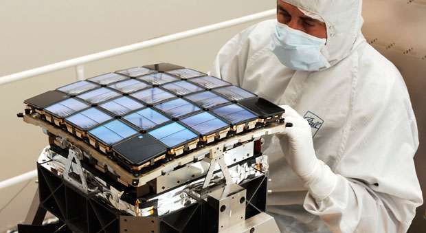

Time series processes: transient
supernovae
stellar “activity”
novae
gamma-ray bursts

detection, identification/classification,
automatic triggers
estimate parameters:
       duration, fluence
       profile shape
       multi- comparison
                            [see RS discussion meeting in April]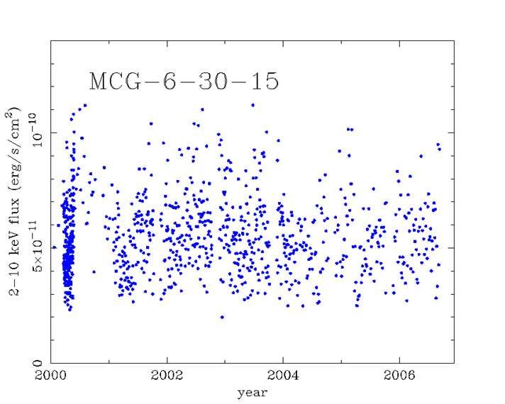

Time series processes: stochastic

 accreting systems (neutron stars, black holes), jets

 cannot predict (time series) data exactly

 statistical comparison between data and model
 to infer physics of system

Data in astronomy

Data in astronomy

Astronomy is observational (not experimental)
Limited to light received (but see Neil Cornish’s talk later)

      images: position on the sky (2 dimensions)
      wavelength: “spectrum” (photon energy)
      polarization
      time “light curves”
      combination of the above

Time series in astronomy

Gapped/irregular data
     Diurnal & monthly cycles
     satellite orbital cycles
     telescope allocations
measurement errors & heteroscedastic
     Signal-to-noise ratio
Poisson processes
     Individual (photon) events in X/-ray astronomy

Time series – what the books say
trends and seasonal components
autoregressive and moving average processes (ARMA)
forecasting
Kalman filters
state-space models
auto/cross-correlation
spectral methods
…and so on

mostly for even sampling, no (or Normal) “errors”
Astronomers more interested in modelling than forecasting

stochastically variable objects
interesting: neutron stars, black holes, turbulent
inflows/outflows, etc.
too small to image ( arcsec)
difficult to measure or interpret polarization
only information from photons(, t)
                                                  physics model

-modelling deterministic
                                observation                          statistical
                               data reduction                       predictions

t-modelling mixed/stochastic

                                    statistical                     model
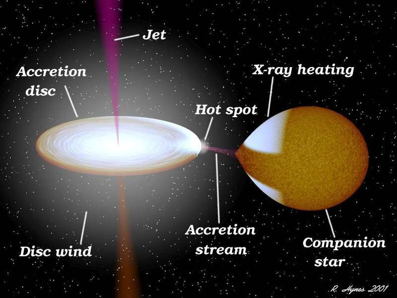
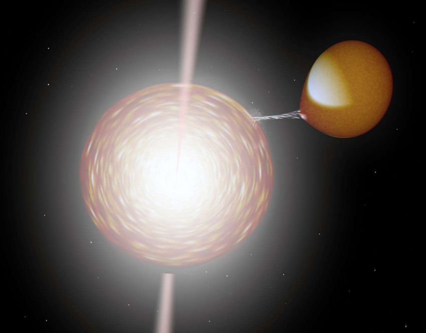
                                   summaries                      comparison

Neutron star
  rotation  few ms

                                       binary system
                                      period  hr-days
inner radius
 orbit  ms           radial inflow
                       sec-weeks

data from RXTE (1996-2012)

Neutron star X-ray binary 4U1608-52
       ~daily monitoring with All-Sky Monitor (ASM)

             1998-03

Neutron star X-ray binary 4U1608-52
       ~daily monitoring with All-Sky Monitor (ASM)

                                          1998-03-27

(X-ray) event list
Table listing each “event” (mostly genuine X-rays) and their recorded properties
e.g. time (detector frame/cycle), channel (event energy), X/Y position, …

               time-t.0 chan           X      Y
                   0.0250     1441    509   517
                   0.0500     4932    510   491
                   0.0875      891    488   507
                   0.1250     5113    494   518
                   0.1375     6985    510   505
                   0.1625     2786    488   476
                   0.2125     2994    504   485
                   0.2500     6566    504   514
                   0.2625     2066    460   513
                   0.2750     1225    492   496
                   ...        …        …     …

(X-ray) data products
                      Select using these

               time-t.0 chan      X     Y
                 0.0250   1441   509   517
                 0.0500   4932   510   491
                 0.0875    891   488   507
                 0.1250   5113   494   518   one, or more,
                 0.1375   6985   510   505   time series
Retain these     0.1625   2786   488   476
                 0.2125   2994   504   485
                 0.2500   6566   504   514
                 0.2625   2066   460   513
                 0.2750   1225   492   496
                 ...      …       …     …

Light curve (time series) product

    “true” flux   s(t)

                  C(ti)
observed
 counts

                          Instrument time
                                       Detector frame i = 1,2,…, N

Light curve (time series) product
                                          expected counts
observed counts/bin
                                        source / background

           x[i ] ~ Pois ( si )  Pois (bi )
                             ti  t

                  si  A        s(t )dt
                               ti

               sensitivity             true source flux

   ignoring possible instrumental non-linearities, etc.

X-ray time series of a transient

                              Type I burst

Data taken with t = 125s resolution, shown binned to t = 1s

X-ray time series of a transient

                              Type I burst
                                                   stochastic
                                                   variations

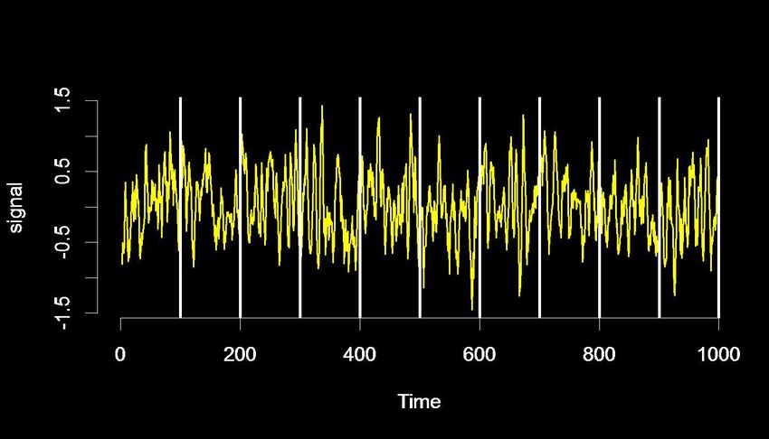
Data taken with t = 125s resolution, shown binned to t = 1s

Standard recipe:
               Power spectrum analysis
                              observed = signal + noise
                                  (not quite right!)

                                    x  sn
Fourier transforms                 X SN
Periodogram          | X |2 | S |2  | N |2  cross  terms
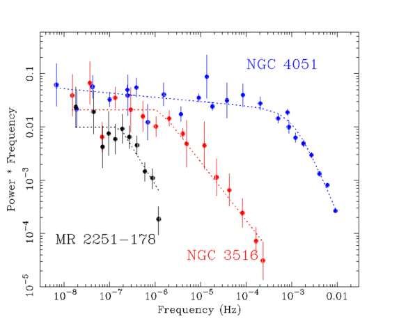
Spectrum              P ( f )  | S |2  | X |2  | N |2

Standard recipe:
                Power spectrum analysis
power density

                         |X|2

                  |N|2
                                     |S|2

                         frequency

Standard recipe

The most popular spectral estimate (in astronomy, at least) is the averaged periodogram,
where periodograms from each of M non-overlapping intervals are averaged.
‘Barlett’s method’ after M. S. Bartlett (1948, Nature, 161, 686-687)

stochastic
              quasi-periodic oscillations (QPOs)

Well-defined peak in power spectrum: f  500-1300 Hz,  f  few Hz
Peak frequency varies on short timescales; strength, width on longer timescales

simple mean vs. “shift and add”
                                           Lorentzian
                                           QPO profile

Shift “short time” periodograms to common centroid frequency
             (small bias on width, power conserved)
    Mendez et al. (1996, ApJ); Barret & Vaughan (2012, ApJ)

An unintentional multi-level model

                                Event times
                  Time     Time     Time     Time     Time
higher level

                  Series   Series   Series   Series   Series
                  f_QPO f_QPO f_QPO f_QPO f_QPO
                 estimate estimate estimate estimate estimate
                   Time series of f_QPO (estimates)
                   Spectrum (estimate) of f_QPO(t)

black hole GRS 1915+105
periodic/stochastic/chaotic/mixed ?

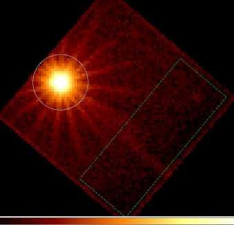
“slow” variations
Kepler mission monitors
10,000s of sources
“continuously”
Q1-Q6 now public…

Kepler light curve of Zw 229-15
problem: how to recover spectrum of very “red” processes?
   (Deeter & Boynton 1982; Fougere 1985; Mushotzky et al. 2011)

     N = 4,125 samples
     t = 29.4 min
     F = 0.1% precision

A message from Captain Data:

                                “More lives have been lost looking at the raw periodogram
                                           than by any other action involving time series!”

                                                    (J. Tukey 1980; quoted by D. Brillinger, 2002)

                                  Fejer kernel

                          f ( Nyq )

            E[ I j ]         F( f
                          f ( Nyq )
                                       j    f ' ) P( f ' ) df '  P( f )  bias[ f ]

even when we can “beat down” the intrinsic fluctuations in the periodogram,
     bias – in the form of leakage and aliasing are difficult to overcome

RXTE monitoring of AGN
problem: what about with low efficiency (uneven) sampling?
                  (Uttley et al. 2002; MNRAS)

RXTE monitoring of AGN
solution: `forward fitting’ through sampling window
              (Uttley et al. 2002; MNRAS)

Forward fitting
‒   Extract time series data x(t)
‒   compute spectrum estimate Pest(f)
‒   define model spectrum P(f;  )
‒   compute dist Pest(f;  ) by Monte Carlo (incl. sampling)
‒   compare data & model – does  look like Pest(f)?

issues:
 - how to estimate spectrum?
 - how to simulate time series data from P(f;  )?
 - how to compare data & model?
 - better in time domain?

Simulation
Time domain methods (e.g. ARMA etc.)

Fourier method         (Ripley 1987; Davies & Harte 1987; Timmer & König 1995)
      –   define: P(f)
      –   compute: E[Re(FT)] = E[Im(FT)] = sqrt(P[f_j]/2)
      –   randomise: FT_j ~ ComplexNorm  sqrt(P[f_j]/2)
      –   invert (FFT): FT  xsim(t_i)

but we are trying to simulate sampling a continuous process
so generate using tsim > Tdata
                                       then resample (subset).
Even so, very fast using FFT. (Assumes linear, Gaussian process)

Bivariate time series

                 Correlation
                      +
                 time delays

             potentially powerful
             causation and scales

bivariate astronomical time series

       
                                        how to recover correlation & delays
y (t )   (t   ) x( ) d    x   (more generally the response function)
                                      from uneven and/or non-simultaneous
Y   X                                time series? when very “red”?

Try for yourself

Sample of astronomical time series (circa 1993)
http://xweb.nrl.navy.mil/timeseries/timeseries.html

Kepler mission archive (continuous optical monitoring)
http://archive.stsci.edu/kepler/

Swift (UK data centre)
http://www.swift.ac.uk/

Plus 1,000s of RXTE time series with