Towards Robust GNSS Positioning and Real-time Kinematic Using Factor Graph Optimization
←
→
Page content transcription
If your browser does not render page correctly, please read the page content below
Accepted in ICRA 2021

 Towards Robust GNSS Positioning and Real-time Kinematic Using
 Factor Graph Optimization

 Weisong Wen and Li-Ta Hsu*

 approach [4] is to use an extended Kalman filter (EKF) [6] to
 Abstract— Global navigation satellite systems (GNSS) are estimate the float solution and the double-differenced (DD)
one of the utterly popular sources for providing globally
 carrier-phase ambiguity bias based on the DD pseudorange
referenced positioning for autonomous systems. However, the
 and carrier-phase measurements. Meanwhile, the LAMBDA
performance of the GNSS positioning is significantly challenged
in urban canyons, due to the signal reflection and blockage from
 algorithm [7] is employed to resolve the integer ambiguity to
buildings. Given the fact that the GNSS measurements are further achieve a fixed solution leading to centimeter-level
highly environmentally dependent and time-correlated, the accuracy. In short, the EKF dominates both the GNSS
conventional filtering-based method for GNSS positioning positioning and the GNSS-RTK positioning, due to the
cannot simultaneously explore the time-correlation among maturity and efficiency of the EKF estimator. Satisfactory
historical measurements. As a result, the filtering-based performance can be obtained for GNSS-RTK (~5 centimeters)
estimator is sensitive to unexpected outlier measurements. In in open-sky areas where the error sources can be dealt with by
this paper, we present a factor graph-based formulation for differential techniques. Unfortunately, the performances of
GNSS positioning and real-time kinematic (RTK). The both the GNSS positioning and GNSS-RTK are significantly
formulated factor graph framework effectively explores the degraded in urban canyons [8] which are mainly due to the
time-correlation of pseudorange, carrier-phase, and doppler outlier measurements, arising from the multipath effects and
measurements, and leads to the non-minimal state estimation of none-line-of-sight (NLOS) [9] receptions caused by the
the GNSS receiver. The feasibility of the proposed method is building reflection and blockage. To mitigate the effects of
evaluated using datasets collected in challenging urban canyons GNSS outliers from NLOS receptions and multipath effects,
of Hong Kong and significantly improved positioning accuracy numerous methods are studied, such as the 3D mapping aided
is obtained, compared with the filtering-based estimator. GNSS (3DMA GNSS) [10-12], the 3D LiDAR aided GNSS
 I. INTRODUCTION positioning [13-16], and the camera aided GNSS positioning
 [1, 17]. However, these methods rely heavily on the
 Global navigation satellite system (GNSS) [1] is currently availability of 3D mapping information or additional sensors.
one of the major sources for providing globally referenced
positioning for autonomous systems with navigation Interestingly, instead of estimating the state of the GNSS
requirements, such as the unmanned aerial vehicle (UAV) [2], receiver mainly based on the observation at the current epoch
autonomous driving vehicles (ADV) [3]. With the increased recursively via the EKF estimator, the recent researches [18-
availability of multi-constellations, the GNSS solution 21] propose the factor graph-based formulation to process the
becomes even more popular. In general, the major positioning GNSS pseudorange measurements and significantly
methods involve GNSS positioning and GNSS real-time improved performance is achieved, compared with the
kinematic (RTK) positioning. conventional EKF. The work [22] by a team from the
 Chemnitz University of Technology was the first paper
 The popular GNSS positioning method is to use the utilizing factor graph optimization (FGO) in GNSS
extended Kalman filter (EKF) [4] to estimate the position, positioning. However, only the pseudorange measurements
velocity, and time (PVT) of the GNSS receiver were considered. Then their continuous works focused on
simultaneously based on the available GNSS measurements. developing a robust model [23-25] for mitigating the effects
General positioning accuracy (5~10 meters) [5] can be of the potential NLOS receptions. Interestingly, a team from
obtained in open sky areas. The remaining error is mainly West Virginia University carried out similar researches [20,
caused by the ionosphere error, troposphere error and satellite 26, 27], applying FGO models to GNSS precise point
clock/orbit biases, etc. To increase the accuracy of the GNSS positioning (PPP) and obtaining significantly improved
positioning, RTK is proposed to perform GNSS positioning results. Inspired by the significant improvement arising from
which can deliver centimeter-level positioning accuracy. The FGO, our previous work [28] extensively evaluated the
GNSS-RTK removes the errors (including the errors performance of the integration of GNSS pseudorange and
mentioned above and the receiver clock offset) using the inertial measurement unit (IMU) using EKF and FGO. Our
double-difference technique based on the observations (e.g. finding showed that the FGO could explore the time-
pseudorange and carrier-phase measurements) received from correlation among the environment dependant GNSS
a reference station. The GNSS-RTK positioning algorithm pseudorange measurements simultaneously, leading to
mainly includes two steps, the float solution estimation, and improved robustness against outliers, compared with the
carrier-phase integer ambiguity resolution. A common EKF-based estimator. However, the potential of FGO in

 Weisong Wen and Li-Ta Hsu are with the Hong Kong Polytechnic
University, Hong Kong. (corresponding author to provide e-mail:
lt.hsu@polyu.edu.hk).
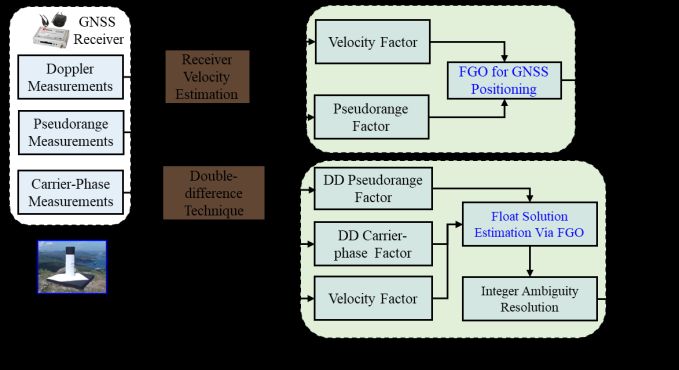
Accepted in ICRA 2021

GNSS-RTK is not explored in the existing work. Meanwhile, (3) The source code for the proposed framework is
the application of full suite GNSS measurements available online. Meanwhile, several datasets are
(pseudorange, Doppler and carrier-phase measurements) in also provided for algorithm development and
FGO is not explored as well. evaluation of researchers. This is the first open-
 source implementation for GNSS positioning and
 To fill this gap, this paper develops a factor graph-based GNSS-RTK using the FGO.
formulation that provides the capability of GNSS positioning
and GNSS-RTK positioning. Regarding the GNSS
positioning, the pseudorange and Doppler measurements are
integrated using FGO where the historical measurements are
utilized simultaneously. Regarding the GNSS-RTK, the DD
pseudorange and carrier-phase measurements are integrated
using FGO where the states are connected using velocity
estimated using Doppler measurements. To the best of the
authors’ knowledge, this is the first integrated framework that
solves the GNSS positioning and GNSS-RTK using the state-
of-the-art FGO. Meanwhile, we open-source the
implementation of the proposed factor graph-based
formulation 1. The rest of the paper is summarized as follows:
the derivation of FGO-based GNSS positioning and GNSS-
RTK methods are described in Section III after the overview Fig. 1 The architecture of the proposed pipeline. The “DD”
of the proposed method is presented in Section II. Then, the stands for the double-difference technique.
experiment is conducted to evaluate the performance of the To make the proposed pipeline clear, the following major
proposed framework in Section IV. Finally, conclusions are notations are defined and followed by the rest of the paper. Be
drawn, together with future work. noted that the state of the GNSS receiver and the position of
 satellites are all expressed in the earth-centered, earth-fixed
 II. OVERVIEW OF THE PROPOSED METHOD (ECEF) frame.
 The architecture of the proposed pipeline is shown in Fig. a) The pseudorange measurement received from a satellite

1 which mainly involves three segments: sensing, modeling, at a given epoch is expressed as , . The subscript
and optimization. The inputs of the system include the raw denotes the GNSS receiver. The superscript denotes
measurements from the GNSS receiver and the observations the index of the satellite.
from the reference station for further GNSS-RTK positioning. b) The Doppler measurement received from satellite at a

The raw GNSS measurements mainly consist of the Doppler, given epoch is expressed as , .
pseudorange, and carrier-phase measurements. In the c) The carrier-phase measurement received from a satellite

modeling segment, the velocity of the GNSS receiver is at a given epoch is expressed as , .
estimated based on the Doppler measurements using the least- d) The position of the satellite at a given epoch is
squares (LS) algorithm. Meanwhile, the double-difference expressed as = ( ,
 , ,
 , , ) .
technique is employed to eliminate satellite and receiver clock e) The velocity of the satellite at a given epoch is
bias, and atmospheric effects based on the observation from expressed as = ( ,
 , ,
 , , ) .
the reference station. In the optimization segment, the f) The position of the GNSS receiver at a given epoch is
solution from GNSS positioning can be obtained by solving
 expressed as , = ( , , , , , , , , ) .
the factor graph formulated by velocity and pseudorange
factor. Meanwhile, the float solution of GNSS-RTK can be g) The velocity of the GNSS receiver at a given epoch is
estimated by solving the factor graph constructed by the DD expressed as , = ( , , , , , , , , ) .
pseudorange, DD carrier-phase, and Doppler measurements. h) The clock bias of the GNSS receiver at a given epoch

Finally, the integer ambiguity is solved using the LAMBDA is expressed as δ , , that with the unit in meters. δ ,
algorithm to achieve a fixed solution. denotes the satellite clock bias by meters.
 i) The position of the base (reference) station is expressed
 The contributions of this paper are listed as follows: as = ( , , , , , ) . The variables ,
 and ,
 (1) This paper develops an FGO-based formulation, denote the pseudorange and range measurements of
 which provides the capability of GNSS positioning carrier-phase from satellite received by the reference
 and RTK positioning. Meanwhile, additional sensor station at epoch .
 measurements, such as LiDAR odometry, can be
 III. METHODOLOGY
 easily integrated into our framework.
 (2) We evaluate the performance of our framework A. GNSS Positioning Using Factor Graph Optimization
 using challenging datasets collected in the urban In terms of the measurements from the GNSS receiver,

 canyons of Hong Kong. The results show that the each pseudorange measurement, , , is denoted as follows
 FGO-based GNSS positioning outperforms the one [29].
 from the EKF-based solutions.

 1
 https://github.com/weisongwen/GraphGNSSLib
Accepted in ICRA 2021

 where the variable ℎ denotes the angular velocity of the
 , = , + (δ , − δ , ) + , + , + , (1)

 earth rotation [4]. The variable denotes the speed of the
where , is the geometric range between the satellite and the light. The variable , ,
 denotes the line-of-sight vector

GNSS receiver. , represents the ionospheric delay distance; connecting the GNSS receiver and the satellite (See equation

 , indicates the tropospheric delay distance. , represents (5)). Therefore, the velocity ( , ) of the GNSS receiver can be
the errors caused by the multipath effects, NLOS receptions, estimated via LS [4] based on equations (4) and (5).
receiver noise, antenna phase-related noise. In this paper, the
satellite systems that we used include the global positioning The graph structure of the proposed factor graph for
system (GPS) and BeiDou. Besides, we follow the methods solving the GNSS positioning is shown in Fig. 2. The subscript
 denotes the total epochs of measurements considered in the
used in RTKLIB [4] to model the atmosphere effects ( , and
 FGO. Each state in the factor graph is connected using the
 , ).
 Doppler velocity factor. The state of the GNSS receiver is
 1 2
 Given the Doppler measurement ( , , , , … ) of each represented as follows:
satellite at an epoch , the velocity ( , ) of the GNSS receiver
can be calculated using the LS method [30]. Giving that the = [ r,1 , r,2 , … , , ] (7)
state of the velocity, , is as follows: , = ( , , , , δ , ) (8)

 = ( , , δ̇ , ) (2) where the variable denotes the set states of the GNSS
 receiver from the first epoch to the current . The , denotes
where the , represents the velocity of the GNSS receiver. the state of the GNSS receiver at epoch t which involves the
The variable δ̇ , stands for the receiver clock drift. The position ( , ), velocity ( , ) and receiver clock bias (δ , ).

range rate measurement vector ( , ) at an epoch is
expressed as follows:
 1 2 3
 , = ( , , , , , , … ) (3)
where the denotes the carrier wavelength of the satellite

signal, the , represents the Doppler measurement. The
observation function ℎ (∗) which connects the state and the
Doppler measurements are expressed as follows:
 1
 , + δ̇ , − δ̇1 ,
 2
 , + δ̇ , − δ̇2 ,
 ℎ ( ) = 3 + δ̇ − δ̇3 (4)
 , , ,
 …

 [ , + δ̇ , − δ̇
 , ] Fig. 2 The purple circle denotes the pseudorange factor (e.g
 s
 With
 , = ℎ ( ) + , , ). The blue shaded rectangle represents the Doppler
 velocity factor (e.g ). The yellow shaded circle stands for
where the superscript denotes the total number of satellites the state of the GNSS receiver.
and the variable ω , stands for the noise associated with the

 , . The variable ,
 denotes the expected range rate. The The observation model for GNSS pseudorange
 measurement from a given satellite is represented as follows:
variables δ̇ , and δ̇ , represent the receiver and satellite clock

bias drift. The Jacobian matrix for the observation function
 ,
 = ℎ , ( , , , δ , ) + ω ,

 (9)
ℎ (∗) is denoted as follows:
 with ℎ , ( , , , δ , ) = || − , || + δ ,
 p1
 , −p , , p1
 , −p , , p1
 , −p , ,
 1
 ‖ 1 ‖ 1 ‖ 1
 where the variable ω , stands for the noise associated with the
 − , ‖ − , ‖ − , ‖
 p2 p2 p2
 , . Therefore, we can get the error function ( , ) for a given
 , −p , , , −p , , , −p , ,
 1 satellite measurement , as follows:
 ‖ 2 − , ‖ ‖ 2 − , ‖ ‖ 2 − , ‖
 = (5)
 p3
 , −p , , p3
 , −p , , p3
 , −p , ,
 1

 || , ||2 = || ,

 − ℎ , ( , , , δ , )||2 (10)
 , ,
 ‖ 3 − , ‖ ‖ 3 − , ‖ ‖ 3 − , ‖
 … … … …
 where , denotes the covariance matrix. We calculate the
 p
 , −p , , p
 , −p , , p
 , −p , ,
 1 , based on the satellite elevation angle, signal, and noise
 [‖
 − , ‖ ‖
 − , ‖ ‖
 − , ‖ ]
 ratio (SNR) following the work in [31]. The observation model
where the operator ‖∗‖ is employed to calculate the range for the velocity ( , ) is expressed as follows:
distance between the given satellite and the GNSS receiver.

The expected range rate ,
 for satellite can also be , = ℎ , ( , +1 , , ) +
 , (11)
calculated as follows:
 , ℎ
 , = , ( − , ) +
 (v ,
 p , , + p , v , , −

 p , v , , − v , p , , ) (6)
Accepted in ICRA 2021

 ( , +1, − , , )
 ⁄ , = ( , − , ) − ( , − , ) (16)
 Δ
 ( − ) The variables , and , stand for the carrier-phase
 with ℎ , ( , +1 , , ) = , +1, , , ⁄ measurements received by the reference station. Similarly, the
 Δ
 ( , +1, − , , )⁄ clock bias and atmosphere effects are waived from , .

 [ Δ ] Meanwhile, the , involves the DD ambiguity [4], which

where the , denotes the velocity measurements given by the is to be estimated.
estimation in (2). The variable , denotes the noise The state of the GNSS receiver is represented as follows:
associated with the velocity measurement. The variable Δ
 = [ ,1 , ,2 , … , , ] (17)
denotes the time difference between epoch and epoch + 1.
Therefore, we can get the error function ( , ) for a given
 1
 , = ( , , , , δ , , Δ , 2
 , Δ , −1
 , … , , Δ , ) (18)

velocity measurement , as follows:
 where the variable denotes the set states of the GNSS
 2 2
 ||
 , || = || , − ℎ , ( , +1 , , )|| (12) receiver from the first epoch to the current . The , denotes
 , ,
 the state of the GNSS receiver at epoch t which consists of

where , denotes the covariance matrix. Therefore, the position ( , ), velocity ( , ) and the DD ambiguities. The
objective function for the GNSS positioning using FGO is −1
 variable Δ , denotes the DD carrier-phase ambiguity bias
formulated as follows: corresponding to satellite − 1. In other words, each DD
 2 2 carrier-phase measurement involves a specific ambiguity bias.
 ∗ = arg min ∑ , ||
 , || + || , || (13)
 , , The graph structure for estimating the float solution of the
 GNSS-RTK is shown in Fig. 3. The yellow shaded circle
The variable ∗ denotes the optimal estimation of the state sets, denotes the state of the GNSS receiver. The purple and red
which can be estimated by solving the objective function (13). circles represent the DD pseudorange and carrier-phase factor,
B. GNSS-RTK Using Factor Graph Optimization respectively. Both the DD pseudorange and carrier-phase
 measurements connect the state of the GNSS receiver and the
 In terms of the measurements from the GNSS receiver, position of the reference station. The blue shaded rectangle

each carrier-phase measurement, , , is written as follows denotes the Doppler velocity factor which is identical to the
[29]. one in GNSS positioning (see Section III-A). The green
 shaded circle denotes the state of the reference station. Be
 , = , + ( , − , ) + , + , + , + noted that the position of the reference station is fixed

 , + , (14) throughout the test.

 where , = ,0, − 0, + ,

where , is the carrier-phase bias. The variable denotes

the carrier wavelength. The variable , denotes the
carrier-phase correction term including antenna phase offsets
and variations, station displacement by earth tides, phase
windup effect, and relativity correction on the satellite clock.
The detailed formulation of the carrier-phase correction can
be found in [4]. The variable ,0, represents the initial phase

of the receiver local oscillator. Similarly, the 0, stands for
the initial phase of the transmitted navigation signal from the

satellite. The variable , denotes the carrier-phase integer

ambiguity. , represents the errors caused by the multipath
effects, NLOS receptions, receiver noise, antenna delay.

 The DD pseudorange measurement ( , ) of satellite is
formulated as follows [4]: Fig. 3 The graph structure for estimating the float solution of

 , = ( , − , ) − ( , − , ) (15) the GNSS-RTK.
The variable ,
 and , stands for the pseudorange Therefore, the observation model for the DD pseudorange

measurements received by the reference station which is measurement ( , ) is expressed as follows:
denoted by the subscript “ ”. Generally, the satellite with the
 ,
 = ℎ , , ( , , ,
 (19)
 , ) + ω , ,
highest elevation angle tends to involve the lowest multipath
and NLOS errors. Therefore, the satellite , with the highest
 ℎ , , ( , , ,
 , ) = (|| , − || − || −
elevation angle, is selected as the master satellite. After
 ||) − (|| , − || − || −

 ||) (20)
applying the DD process to the pseudorange measurements,

the derived , is free of the clock bias and atmosphere The variable ω , , denotes the noise associated with the

effects [4]. Similarly, the DD carrier-phase measurement , . The function ℎ , , (∗) denotes the observation

( , ) of satellite is formulated as follows [4]: function connecting the state of the GNSS receiver and the DD
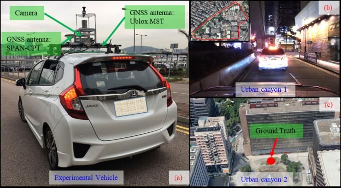
Accepted in ICRA 2021

measurement , . Therefore, the error factor for the DD can get fixed in the less urbanized area) using the same sensor
pseudorange measurement as follows: setup as the one in urban canyon 1. We run the proposed
 framework using a high-performance laptop computer with an

|| , , ||2
 = || ,
 − ℎ , , ( , , , 2
 , )|| Intel i7-9750K at 2.60GHz and 32GB RAM. For the GNSS
 , , , ,
 (21) positioning evaluation, we compare the following methods:

 (1) WLS [4]: GNSS positioning is based on the
The variable , ,
 stands for the covariance associated with pseudorange using WLS via RTKLIB.

the , . Similarly, the observation model for the DD carrier-
phase measurement is expressed as follows: (2) EKF: GNSS positioning based on the integration of
 pseudorange and velocity from Doppler

 , = ℎ , , ( , , ,
 , ) + ω , , (22) measurements using the EKF estimator.

 ℎ , , ( , , , (3) FGO: GNSS positioning based on the integration of
 , ) = (|| , − || − || −
 pseudorange and velocity from Doppler

 ||) − (|| , −
 || − || − ||) + Δ , (23) measurements using FGO.

The variable ω , , denotes the noise associated with the For the GNSS-RTK evaluation, we compare the

 , . The variable Δ , denotes the DD ambiguity of the following methods:
carrier-phase measurement. Therefore, the error factor for the (1) RTK-EKF [4]: GNSS-RTK positioning based on
DD carrier-phase measurement is as follows: the DD pseudorange and carrier-phase
 measurements using the EKF estimator via RTKLIB.

 || , , ||2
 = || , −
 , ,
 2 (2) RTK-FGO: GNSS-RTK positioning based on the
 ℎ , , ( , , ,
 , )|| (24)
 , , DD pseudorange, Doppler measurement, and

The variable , , stands for the covariance associated with carrier-phase measurements using the FGO. Be
 noted that the integer ambiguity is resolved using the
the , . Therefore, the objective function for the float
 LAMBDA algorithm.
solution estimation of GNSS-RTK using FGO is formulated
as follows: The positioning performance of the listed five methods is
 2 2
 evaluated in the east, north, and up (ENU) frame. As the
 ∗ = arg min ∑ , ||
 , || + || , , || + GNSS positioning in the vertical direction is highly unreliable
 , , ,

 due to the satellite geometry, only the horizontal positioning

 || , , ||2 (25)
 , , is evaluated.
The variable ∗ denotes the optimal estimation of the state sets.
Therefore, the float solution for GNSS-RTK at the current
epoch can be obtained by solving the above objective function
(25). After obtaining the float solution of the GNSS-RTK
using FGO, an ambiguity resolution algorithm is used to

estimate the fixed solution. The variable Δ , should be an
integer value when the carrier-phase measurement is free from
the noise. This paper makes use of the popular LAMBDA
algorithm [32] to solve the integer ambiguity resolution
problem. Due to the page's limitations, the detailed
presentation of the employed LAMDA algorithm can be found
online 2.

 IV. EXPERIMENT RESULTS AND DISCUSSIONS Fig. 4 The sensor setup of the experimental vehicle and
 evaluated scenarios. (a) sensor setup of the experimental
 Two experimental evaluations are conducted to evaluate vehicle. (b) the experimental scene with tall buildings in
the performance of the proposed framework. The urban canyon 1. (c) the experimental scene in urban canyon 2.
experimental vehicle is shown on the left side of the following
Fig. 4. To validate the effectiveness of the proposed GNSS A. Evaluation of the Proposed GNSS Positioning
positioning using FGO, we collected data in a challenging The positioning error of GNSS positioning in the
urban canyon 1 (see Fig. 4-(b)) with numerous multipath evaluated dataset is shown in the following Table 1. A mean
effects and NLOS receptions. During the test, a u-blox M8T of 17.39 meters is obtained using WLS with a standard
GNSS receiver is used to collect raw single-frequency GPS deviation (STD) of 16.01 meters. Meanwhile, the maximum
and BeiDou measurements at a frequency of 1 Hz. Besides, error reaches 94.43 meters. After applying the EKF to
the NovAtel SPAN-CPT, a GNSS RTK/INS (fiber optic integrate the pseudorange measurements, and the velocity of
gyroscopes) integrated navigation system is used to provide the GNSS receiver derived from the Doppler measurement,
the ground truth. To validate the effectiveness of the proposed the mean error decreases to 13.61 meters based on EKF.
GNSS-RTK method using FGO, we collect the other static Meanwhile, the STD is also reduced slightly to 15.19 meters.
dataset in a less urbanized area (see Fig. 4-(c), the GNSS-RTK However, the maximum error still reaches about 89 meters
 2
 https://github.com/weisongwen/GraphGNSSLib
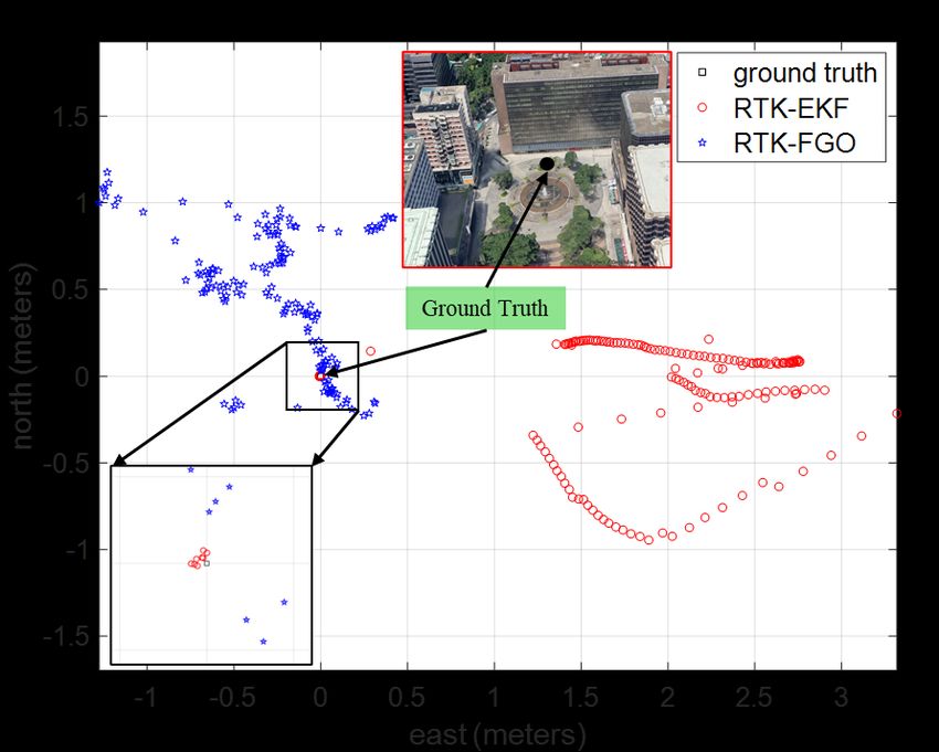
Accepted in ICRA 2021

due to the numerous unexpected outlier measurements. The Fig. 6 shows the trajectories using the two different
mean error decreases to only 9.45 meters after applying the methods and ground truth. The more accurate trajectory is
FGO with a significantly decreased STD of 8.06 meters. achieved using RTK-FGO with the help of velocity
Meanwhile, the maximum error decreases to only 31.94 measurements, compared with the RTK-EKF. We can see
meters. The significantly improved positioning accuracy from Table 2 that the RTK-EKF gets a fixed rate of 4.4% in
shows the effectiveness of the proposed framework based on the evaluated urban canyon 2. Interestingly, the fixed rate of
FGO. the proposed RTK-FGO is slightly decreased to 3.8%. The
 reason is that the proposed RTK-FGO did not consider the
 Fig. 5 shows the trajectories using three different cycle slip detection [33] and the ambiguity is solved
methods and ground truth. The black curve denotes the independently in each epoch.
ground truth trajectory provided by the SPAN-CPT. The
smoother trajectory is achieved using EKF with the help of Table.2 Positioning performance of the GNSS-RTK
velocity measurements, compared with the WLS. However,
the trajectory can still deviate significantly from the ground All data RTK-EKF RTK-FGO
truth trajectory in some epochs. With the help of the proposed MEAN (m) 2.01 0.64
framework, a smoother trajectory is obtained almost STD (m) 0.67 0.40
throughout the test. MAX (m) 3.33 1.70
Table.1 GNSS positioning performance using the three listed Availability 100% 100%
 methods Fixed Rate 4.4% 3.8%
 All data WLS EKF FGO
 MEAN (m) 17.39 13.61 9.45
 STD (m) 16.01 15.19 8.06
 MAX (m) 94.43 88.97 31.94
 Availability 100% 100% 100%

 (b)

 (a)

 (c)

 Fig. 6 Positioning results of two methods RTK-EKF (red dots)
 and RTK-FGO (blue dots).

 V. CONCLUSION AND FUTURE WORK

Fig. 5 Trajectories of three methods WLS (red), EKF (green), This paper developed a factor graph-based formulation,
 that enables the capability of the two most popular positioning
and FGO (blue). The x-axis and y-axis denote the east and methods, the GNSS positioning, and GNSS-RTK. We
north directions, respectively. evaluate the proposed framework using the dataset collected
B. Evaluation of the Proposed GNSS-RTK in the urban canyons of Hong Kong. The results show that the
 During the static test in urban canyon 2, the Doppler proposed method can effectively help to mitigate the effects
velocity measurements are employed to connects the of GNSS outlier measurements, deriving improved accuracy
consecutive states. The positioning accuracy of GNSS-RTK both in GNSS positioning and GNSS-RTK positioning. The
in the evaluated dataset is shown in the following Table 2. Be cycle slip detection will be applied to the integer ambiguity
noted that the float solution is recorded when the fixed resolution to improve the fixed rate in the future. Moreover,
solution is not available. A mean of 2.01 meters is obtained achieving a fixed solution for positioning autonomous
using RTK-EKF with an STD of 0.67 meters. Meanwhile, the systems in the urban canyon is still a challenging problem to
maximum error reaches 3.33 meters. The mean error solve, we will also explore adding more sensors to the
decreases to only 0.64 meters after applying the RTK-FGO proposed framework to increase the fixed rate of GNSS-RTK.
with a slightly decreased STD of 0.40 meters. Meanwhile, the
maximum error decreases to only 1.70 meters. The improved ACKNOWLEDGMENT
positioning accuracy shows that the proposed RTK-FGO The authors acknowledge the ROS, RTKLIB, and the
method can effectively mitigate the effects of the GNSS provider of OpenStreetMap.
outlier measurements, leading to improved accuracy.
Accepted in ICRA 2021

 REFERENCES [20] R. M. Watson and J. N. Gross, "Robust navigation in GNSS
 degraded environment using graph optimization," arXiv preprint
 arXiv:1806.08899, 2018.
 [21] W. Wen, X. Bai, Y. C. Kan, and L.-T. Hsu, "Tightly Coupled
[1] T. Suzuki, M. Kitamura, Y. Amano, and T. Hashizume, "High-
 GNSS/INS Integration via Factor Graph and Aided by Fish-Eye
 accuracy GPS and GLONASS positioning by multipath
 Camera," IEEE Transactions on Vehicular Technology, vol. 68,
 mitigation using omnidirectional infrared camera," in 2011 IEEE
 no. 11, pp. 10651-10662, 2019.
 International Conference on Robotics and Automation, 2011, pp.
 [22] N. Sünderhauf and P. Protzel, "Towards robust graphical models
 311-316: IEEE.
 for GNSS-based localization in urban environments," in
[2] M. Saska, J. Vakula, and L. Přeućil, "Swarms of micro aerial
 International Multi-Conference on Systems, Signals & Devices,
 vehicles stabilized under a visual relative localization," in 2014
 2012, pp. 1-6: IEEE.
 IEEE International Conference on Robotics and Automation
 [23] T. Pfeifer and P. Protzel, "Expectation-maximization for adaptive
 (ICRA), 2014, pp. 3570-3575: IEEE.
 mixture models in graph optimization," in 2019 International
[3] G. Wan et al., "Robust and precise vehicle localization based on
 Conference on Robotics and Automation (ICRA), 2019, pp. 3151-
 multi-sensor fusion in diverse city scenes," in 2018 IEEE
 3157: IEEE.
 International Conference on Robotics and Automation (ICRA),
 [24] T. Pfeifer and P. Protzel, "Robust sensor fusion with self-tuning
 2018, pp. 4670-4677: IEEE.
 mixture models," in 2018 IEEE/RSJ International Conference on
[4] T. Takasu and A. Yasuda, "Development of the low-cost RTK-
 Intelligent Robots and Systems (IROS), 2018, pp. 3678-3685:
 GPS receiver with an open source program package RTKLIB," in
 IEEE.
 International symposium on GPS/GNSS, 2009, pp. 4-6:
 [25] T. Pfeifer, S. Lange, and P. Protzel, "Dynamic Covariance
 International Convention Center Jeju Korea.
 Estimation—A parameter free approach to robust Sensor Fusion,"
[5] J. Breßler, P. Reisdorf, M. Obst, and G. Wanielik, "GNSS
 in 2017 IEEE International Conference on Multisensor Fusion
 positioning in non-line-of-sight context—A survey," in Intelligent
 and Integration for Intelligent Systems (MFI), 2017, pp. 359-365:
 Transportation Systems (ITSC), 2016 IEEE 19th International
 IEEE.
 Conference on, 2016, pp. 1147-1154: IEEE.
 [26] R. M. Watson, J. N. Gross, C. N. Taylor, and R. C. Leishman,
[6] S. Thrun, "Probabilistic robotics," Communications of the ACM,
 "Uncertainty Model Estimation in an Augmented Data Space for
 vol. 45, no. 3, pp. 52-57, 2002.
 Robust State Estimation," arXiv preprint arXiv:1908.04372, 2019.
[7] P. Teunissen, "The LAMBDA method for the GNSS compass,"
 [27] R. M. Watson, J. N. Gross, C. N. Taylor, and R. C. Leishman,
 Artificial Satellites, vol. 41, no. 3, pp. 89-103, 2006.
 "Robust Incremental State Estimation through Covariance
[8] N. Kubo and C. Dihan, "Performance evaluation of RTK-GNSS
 Adaptation," arXiv preprint arXiv:1910.05382, 2019.
 with existing sensors in dense urban areas," J. Geodesy Geomat.
 [28] W. Wen, T. Pfeifer, X. Bai, and L.-T. Hsu, "Comparison of
 Eng, vol. 1, pp. 18-28, 2014.
 Extended Kalman Filter and Factor Graph Optimization for
[9] L.-T. Hsu, "Analysis and modeling GPS NLOS effect in highly
 GNSS/INS Integrated Navigation System," arXiv preprint
 urbanized area," GPS solutions, vol. 22, no. 1, p. 7, 2018.
 arXiv:2004.10572, 2020.
[10] L.-T. Hsu, Y. Gu, and S. Kamijo, "3D building model-based
 [29] E. Kaplan and C. Hegarty, Understanding GPS: principles and
 pedestrian positioning method using GPS/GLONASS/QZSS and
 applications. Artech house, 2005.
 its reliability calculation," (in English), GPS Solutions, vol. 20, no.
 [30] B. Hofmann-Wellenhof, H. Lichtenegger, and E. Wasle, GNSS–
 3, pp. 413–428, 2016.
 global navigation satellite systems: GPS, GLONASS, Galileo, and
[11] P. D. Groves and M. Adjrad, "Likelihood-based GNSS
 more. Springer Science & Business Media, 2007.
 positioning using LOS/NLOS predictions from 3D mapping and
 [31] A. M. Herrera, H. F. Suhandri, E. Realini, M. Reguzzoni, and M.
 pseudoranges," GPS Solutions, vol. 21, no. 4, pp. 1805-1816,
 C. de Lacy, "goGPS: open-source MATLAB software," GPS
 2017.
 solutions, vol. 20, no. 3, pp. 595-603, 2016.
[12] H.-F. Ng, G. Zhang, and L.-T. Hsu, "A computation effective
 [32] P. Teunissen, "Theory of integer equivariant estimation with
 range-based 3D mapping aided GNSS with NLOS correction
 application to GNSS," Journal of Geodesy, vol. 77, no. 7-8, pp.
 method," The Journal of Navigation, pp. 1-21, 2020.
 402-410, 2003.
[13] W. Wen, G. Zhang, and L.-T. Hsu, "Exclusion of GNSS NLOS
 [33] T. Takasu and A. Yasuda, "Cycle slip detection and fixing by
 receptions caused by dynamic objects in heavy traffic urban
 MEMS-IMU/GPS integration for mobile environment RTK-
 scenarios using real-time 3D point cloud: An approach without
 GPS," in Proc. 21st Int. Tech. Meeting of the Satellite Division of
 3D maps," in Position, Location and Navigation Symposium
 the Institute of Navigation (ION GNSS 2008), Savannah, GA,
 (PLANS), 2018 IEEE/ION, 2018, pp. 158-165: IEEE.
 2008, pp. 64-71: Citeseer.
[14] W. Wen, G. Zhang, and L.-T. Hsu, "GNSS NLOS Exclusion
 Based on Dynamic Object Detection Using LiDAR Point Cloud,"
 IEEE Transactions on Intelligent Transportation Systems, 2019.
[15] W. Wen, G. Zhang, and L. T. Hsu, "Correcting NLOS by 3D
 LiDAR and building height to improve GNSS single point
 positioning," Navigation, vol. 66, no. 4, pp. 705-718, 2019.
[16] W. Wen, "3D LiDAR Aided GNSS and Its Tightly Coupled
 Integration with INS Via Factor Graph Optimization," in
 Proceedings of the 33rd International Technical Meeting of the
 Satellite Division of The Institute of Navigation (ION GNSS+
 2020), 2020, pp. 1649-1672.
[17] X. Bai, W. Wen, and L.-T. Hsu, "Using Sky-Pointing Fish-eye
 Camera and LiDAR to Aid GNSS Single Point Positioning in
 Urban Canyons (submitted)," IET Intelligent Transport Systems,
 2019.
[18] N. Sünderhauf, M. Obst, G. Wanielik, and P. Protzel, "Multipath
 mitigation in GNSS-based localization using robust
 optimization," in 2012 IEEE Intelligent Vehicles Symposium,
 2012, pp. 784-789: IEEE.
[19] W. Li, X. Cui, and M. Lu, "A robust graph optimization
 realization of tightly coupled GNSS/INS integrated navigation
 system for urban vehicles," Tsinghua Science and Technology,
 vol. 23, no. 6, pp. 724-732, 2018.
You can also read