UC Santa Barbara GIScience 2021 Short Paper Proceedings
←
→
Page content transcription
If your browser does not render page correctly, please read the page content below
UC Santa Barbara
GIScience 2021 Short Paper Proceedings

Title
Examining geographical generalisation of machine learning models in urban analytics
through street frontage classification and house price regression

Permalink
https://escholarship.org/uc/item/1690j3zc

Authors
Law, Stephen
Jeszenszky, Peter
Yano, Keiji

Publication Date
2021-09-01

DOI
10.25436/E2VC71

Peer reviewed

 eScholarship.org                             Powered by the California Digital Library
                                                              University of California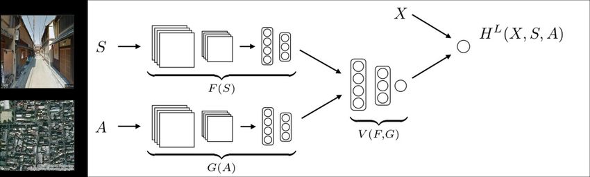
1   Examining geographical generalisation of machine
 2   learning models in urban analytics through street
 3   frontage classification and house price regression
 4   Stephen Law
 5   UCL Geography, UK
 6   The Alan Turing Institute, UK
 7   stephen.law@ucl.ac.uk

 8   Péter Jeszenszky
 9   University of Bern, Switzerland
10   peter.jeszenszky@csls.unibe.ch

11   Keiji Yano
12   Ritsumeikan University, Japan
13   yano@lt.ritsumei.ac.jp

14         Abstract
15   The use of machine learning models (ML) in spatial statistics and urban analytics is increasing.
16   However, research studying the generalisability of ML models from a geographical perspective had
17   been sparse, specifically on whether a model trained in one context can be used in another. The
18   aim of this research is to explore the extent to which standard models such as convolutional neural
19   networks being applied on urban images can generalise across different geographies, through two
20   tasks. First, on the classification of street frontages and second, on the prediction of real estate
21   values. In particular, we find in both experiments that the models do not generalise well. More
22   interestingly, there are also differences in terms of generalisability within the first case study which
23   needs further exploration. To summarise, our results suggest that in urban analytics there is a need
24   to systematically test out-of-geography results for this type of geographical image-based models.

28    1     Introduction

29   Machine learning (ML) methods such as convolutional neural networks (CNN ) have achieved
30   human-level accuracy in many computer vision tasks such as scene recognition, object
31   detection and image segmentation [1, 16]. This level of computer intelligence has led to
32   advances in intelligent transportation, medical imaging, robotics and in our case urban
33   analytics. For example, these methods have been used to estimate socio-economic profiles
34   [3], predict the perceived safety of streets [12, 20], classify street frontage quality [10] and to
35   estimate property prices [9]. A key limitation is the lack of research on how machine learning
36   methods on urban scenes generalise geographically. If a model trained in one context can be
37   successfully used in another then there is less data annotations and thus more generalisable
38   and spatially reproducible models[7]. To address this concern, this exploratory research
39   aims to study whether standard machine learning models (CNN ) on urban images can
40   generalise over vastly different geographical context on two common tasks in ML, namely an
41   image-based classification task and a regression task.
2 GeoML generalisation
42 1.1 Related work on the analysis of urban imagery
43 Diving deeper into the analysis of urban imagery, Salesses et al. [18] collected data on the
44 perception of safety from street image, using a crowd-sourced survey to study the number
45 of homicides in US cities. Naik et al. [12] expanded on this by fitting a regression model
46 [20] to predict perceived safety and liveliness. Recently, Law et al. [10] have constructed a
47 CNN model to infer whether the street has active frontages or not. While, Law et al. [9],
48 used both street level and aerial images to estimate house price directly using a CNN-based
49 hedonic price model for the Greater London area.
50 Despite the increase in research using urban imagery, studying how these models generalise
51 geographically has been limited. Naik et al. [12] found that their urban computer vision
52 models generalise poorly between the East and the West Coast in the United States. In an
53 attempt to obtain a global model, [2] extended the Place Pulse dataset to 56 cities around the
54 world. Using this dataset, Dubey et al. [2] trained a CNN model that can predict pairwise
55 perceived safety from a pair of input StreetView images. Subsequently, they used this global
56 model to make a similar prediction for six additional cities and found the prediction score
57 conforms well through visual inspections. Our research main novelty is to study the concept
58 of ML model generalisation from a geographical perspective; through a classification task
59 (street frontage classification) and a regression task (real estate value prediction). For brevity,
60 we term these case study 1 and case study 2.
61 2 Method and Materials
62 2.1 Case study 1: Street Frontage Classification
63 The quality of street frontages is an important factor in urban design, as it contributes
64 to the safety and liveliness of the public space [5]. In this study, active street frontage is
65 defined as having windows and doors on the ground floor of the building frontage, as opposed
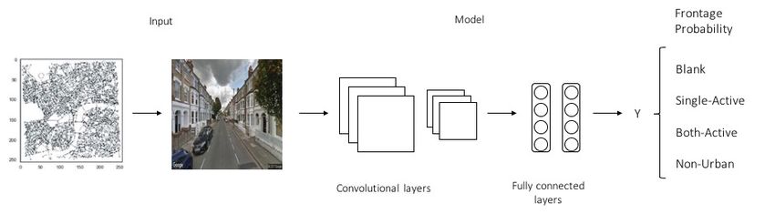
66 to blank walls [14]. In case study 1, we investigate the extent to which a street frontage
67 classification model which classifies a Google StreetView image into four frontage categories;
68 blank frontage, single-side active frontage , both-sides active frontage and non-urban frontage
69 can generalise to different geographical contexts.
70 Front-facing street images were firstly collected using Google StreetView API [4] following
71 similar procedures to [10]. In total we downloaded 109,419 front-facing StreetView images
72 in London, 5972 images in Kyoto, 2157 images in Hong Kong, 6012 images in Tokyo, 2746
73 images in Barcelona, 4157 images in San Francisco, 3143 images in NYC and 4434 images in
74 Paris. In London, 10,000 images were manually labelled in order to train the initial model,
75 and in each of the seven cities, 350 images were labelled.
76 Following [10], we train a Street-Frontage-Net classifier SF N (·) that takes Streetview
77 image S as input and returns a probability vector for each frontage class k. SF N uses a
78 pretrained VGG16 architecture [19] from Imagenet as a feature extractor. These features
79 then get pushed through a pair of fully-connected layers where a Softmax activation function
80 is used in the final layer to estimate the probability of the four frontage class for an input
81 image. We then split the dataset and use 60% for training, 20% for validation and 20% for
82 testing and train the SF N using stochastic gradient descent (lr=0.001 ). We minimise the
PM
83 categorical cross entropy loss function; H(y, ŷ) = − k=1 yk log(ŷk ) where ŷk is the predicted
84 probability for class k with M classes, and yk is the true probability for the same class. For
85 more details of the data collection process and architecture, please see Law et al. [10].
86 For case study 1, we study the extent to which the SF N model trained in London canLaw, Jeszenszky, Yano 3
Figure 1 Case Study 1: Street frontage classification model [10]
87 generalise across the seven other cities. We report the classification accuracy, or the number
88 of times the prediction of the frontage class matches the four observed frontage classes. Fig
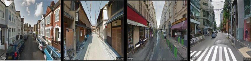
89 2 shows example of the streetview images.
90 2.2 Case study 2: Real estate value prediction
91 In case study 2, we study the extent to which an urban image-based real estate value
92 regression model can generalise between London and Kyoto. We adopt an existing end-to-end
93 methodology akin to [9] that estimates the real estate value from both its location attributes
94 and visual attributes from urban images. To ensure that the cases are more comparable, we
95 construct a parsimonious hedonic price model to predict the real estate value (price per sqm)
96 based on location and visual attributes at the street segment level.
Figure 2 Examples of Google Street images from left to right, London, Kyoto, Paris and Tokyo.
97 In terms of the property attributes, we use the UK Land Registry Price Paid dataset [15],
98 coupled with detail attributes from Nationwide Housing Society [13] to form the house price
99 data in London. For Kyoto, we used the Rosenka dataset, which is a road valuation dataset
100 from 2012 which gives the mean land price per sqm for each street [17]. We calculate the
101 mean house price sqm at the street-level from the London data in order to match with the
102 Kyoto data. In terms of the location attributes, we calculate two street network accessibility
103 measures which are commonly included in house price models [9]. Specifically, we calculate
104 closeness centrality, which measures the inverse average distance to all other streets in the
105 network as a proxy for capturing geographic accessibility, and betweenness centrality, which
106 measures the number of shortest paths overlap from all streets to all streets as a proxy for
107 street hierarchy and congestion of a city [6].
108 In terms of the visual attributes, we used the same front-facing streetview images from
109 case study 1 for London. Following [9], we have also collected aerial images using Microsoft
110 Bing Maps API [11] for both London and Kyoto. In total, the dataset consists of 39, 346
111 aerial image samples in London and 7, 040 in Kyoto. The output variable, price per sqm,
112 is log transformed, which is a standard procedure in the literature [9], while all the input4 GeoML generalisation
113 attributes are normalised to have a mean of 0 and a standard deviation of 1.
114 Following [9], we train a model H(·) with the streetview and aerial images while controlling
115 for the contribution of the housing attributes. To extract visual features from the StreetView
116 images S and aerial images A, we define two functions F (S) and G(A) which extract features
117 as additional inputs into a hedonic price model. Both networks adopt a VGG-like [19] CNN
118 architecture, where we take the value at the final flattened convolutional layer followed by
119 a pair of fully-connected layers. We then concatenate the output of these two networks
120 followed by two additional fully-connected layers in compressing the feature vectors output
121 of F (S) and G(A) to a visual summary scalar response.
Figure 3 Case study 2: Hedonic price model architecture [9]
122 This visual response can then be included as an additional independent variable in an
OLS model where we can compare a standard linear model; H L (X) = β0 + βX + , which
P
123
124 only uses the housing attributes X, to an extended model H L (X, S, A) that includes the
visual summary response as H L (X, S, A) = β0 + βX + γV (F (S), G(A)) + , where β are
P
125
126 the OLS regression weights for the location attributes, and γ as the weights for the visual
127 summary response. We then split the dataset and use 70% for training, 15% for validation
128 and 15% for testing and train the model using ADAM [8](learning rate=0.001) minimising
129 the mean squared error loss function. For more details of the data collection process and
130 architecture, please see Law et al. [9].
131 The aims of case study 2 are two-fold. First, to test whether the method works in a
132 vastly different context, in this case Kyoto. Second, to test the extent to which the image
133 features trained with the London data can be used and generalised to Kyoto and vice versa.
134 To address both of these aims, we estimated six linear regression models on the testset, each
135 of which are different combinations of housing attributes, and visual attributes of the two
136 cities. Hedonic price models M1 to M3 deliver predictions for London, while models M4
137 to M6 for Kyoto. Model M1 is the baseline hedonic price model for London that includes
138 the housing attributes only. Model M2 is the same as the London-baseline but includes
139 both housing attributes and visual response retrieved from the London-trained-CNN model
140 on London images. Model M3 includes both the housing attributes and visual response
141 retrieved from the Kyoto-trained-CNN model on London images. Model M4 is the baseline
142 hedonic price model for Kyoto that includes the housing attributes only. Model M5 is the
143 same as the Kyoto-baseline but includes both the housing attributes and the visual response
144 retrieved from the Kyoto-trained-CNN model on Kyoto images. Model M6 includes both
145 the housing attributes and the visual response retrieved from London-trained-CNN model on
146 Kyoto images. For each model, we report the adjusted R-squared measures, as a general
147 goodness of fit metric (Table 1).Law, Jeszenszky, Yano 5
148 3 Results and Conclusion
149 Presenting the results of case study 1, Table 1 shows the accuracy of 87.5% for the baseline
150 London model which were used to make inference for the seven other cities namely; Paris at
151 77.26%, New York at 73.30%, Barcelona at 70.48%, San Francisco at 69.43%, Hong Kong at
152 67.78%, Kyoto at 56.25% and Tokyo at 52.20%. These results confirm a naive assumption
153 that architecturally more similar cities can achieve a higher accuracy.
Table 1 Case study 1 results
Cities Accuracy Table 2 Case study 2 results
London 87.50%
Paris 77.26% Location Model adjR2
NYC 73.30% London M1 (noVis) 63.90%
Barca 70.48% London M2 (LonVis) 71.6%
SFO 69.43% London M3 (KyoVis) 63.90%
HKG 67.78% Kyoto M4 (noVis) 29.30%
Kyoto 56.25% Kyoto M5 (KyoVis) 42.40%
Tokyo 52.20% Kyoto M6 (LonVis) 29.90%
154 Table 2 shows the goodness of fit (adjR2) results for case study 2, comparing the six
155 regression models. The results show that the goodness of fit improved from 63.9% (M1
156 London baseline) to 71.6% for London (M2) and from 29.3% (M4 Kyoto baseline)to 42.4%
157 for Kyoto (M5) when including its own visual response. However, there is no improvement
158 when using the Kyoto visual response in the London hedonic price model (M3) and a
159 negligible improvement when using the London visual response in the Kyoto model (M6).
160 To summarise, this exploratory research studied whether a standard (ML) model such as
161 CNN can generalise well geographically for two tasks, classification of street frontages and
162 prediction of real estate values. For both tasks, we have found poor model generalisability
163 across different geographical contexts, albeit we also noticed differences in generalisability.
164 For example in case study 1, we found that the street frontage classification model trained
165 using only the London StreetView images generalises better to cities that are architecturally
166 more similar to London, such as Paris (eg. western style, bricks, stones), and poorer for cities
167 that are architecturally dissimilar, such as Kyoto (eg. eastern style, wood, concrete). In case
168 study 2, we confirm that response extracted from urban images can improve existing real
169 estate value predictions for both London and Kyoto. However, we also found that the visual
170 response learnt from one context cannot be easily generalised to another context, echoing
171 the result of previous research [12]. A number of limitations remain, including the lack of
172 samples and the lack of cross cities analysis. For example, whether a model trained in other
173 cites can generalise to London and whether a model trained in a subset or all of the cities
174 can generalise better (eg. Dubey et al. 2016 [2]). There were also a lack of case studies
175 in the house price prediction tasks due to the difficulty in collecting comparable data in
176 different cities. From a geographical perspective, future research could also consider how
177 spatial dependence differs across different geographies for this type of model. To end, these
178 results suggest that there is a need to systematically test ML models in different geographies
179 as well as the need for human evaluation experiments to study these differences in detail for
180 future research. Even though the results are not conclusive, it serves as an initial exploration
181 on ML models generalisation from a geographical perspectives.6 GeoML generalisation
182 References
183 1 Vijay Badrinarayanan, Alex Kendall, and Roberto Cipolla. Segnet: A deep convolutional
184 encoder-decoder architecture for image segmentation, 2016. arXiv:1511.00561.
185 2 A Dubey, N Naik, D Parikh, R Raskar, and C Hidalgo. Deep learning the city : Quantifying
186 urban perception at a global scale. European Conference on Computer Vision (ECCV), 2016.
187 3 T Gebru, J Krause, Y Wang, D Chen, J Deng, E Aiden, and F Li. Using deep learning and
188 google street view to estimate the demographic makeup of neighbourhoods across the united
189 states. PNAS, 2017.
190 4 Google. https://www.maps.google.com/, 2018. Google StreetView retrieved in 2018.
191 5 E Heffernan, T Heffernan, and W Pan. The relationship between the quality of active frontages
192 and public perceptions of public spaces. Urban Design international, 2014.
193 6 B. Hillier and O. Shabaz. An evidence based approach to crime and urban design – Or can
194 we have vitality, sustainability and security all at once? http : //spacesyntax.com/wp −
195 content/uploads/2011/11/Hillier − SahbazA n − evidence − based − approach0 10408.pdf ,
196 visited : June2014, 2005.
197 7 Peter Kedron, Amy E Frazier, Andrew B Trgovac, Trisalyn Nelson, and A Stewart Fother-
198 ingham. Reproducibility and replicability in geographical analysis. Geographical Analysis,
199 53(1):135–147, 2021.
200 8 Diederik P. Kingma and Jimmy Ba. Adam: A method for stochastic optimization, 2014.
201 arXiv:1412.6980.
202 9 Stephen Law, Brooks Paige, and Chris Russell. Take a look around: using street view and
203 satellite images to estimate house prices. ACM Transactions on Intelligent Systems and
204 Technology (TIST), 10(5):1–19, 2019.
205 10 Stephen Law, Chanuki Illushka Seresinhe, Yao Shen, and Mario Gutierrez-Roig. Street-
206 frontage-net: urban image classification using deep convolutional neural networks. International
207 Journal of Geographical Information Science, 0(0):1–27, 2018. arXiv:https://doi.org/10.
208 1080/13658816.2018.1555832, doi:10.1080/13658816.2018.1555832.
209 11 Microsoft. https://www.microsoft.com/en-us/maps/choose-your-bing-maps-api, 2018.
210 Bing Aerial Maps retrieved in 2018.
211 12 N. Naik, J. Philipoom, R. Raskar, and C.A. Hidalgo. Streetscore - predicting the perceived
212 safety of one million streetscapes. In CVPR Workshop on Web-scale Vision and Social Media,
213 2014.
214 13 Nationwide. Auxiliary housing attributes. permission of use from london school of economics.
215 https://www.nationwide.co.uk/, 2012.
216 14 Office of the Deputy Prime Minister. Safer Places: The Planning System and Crime Prevention.
217 Home Office, 2005.
218 15 Land Registry. https://www.gov.uk/search-house-prices, 2017.
219 16 Shaoqing Ren, Kaiming He, Ross Girshick, and Jian Sun. Faster r-cnn: Towards real-time
220 object detection with region proposal networks, 2016. arXiv:1506.01497.
221 17 Hadrien Salat, Roberto Murcio, Keiji Yano, and Elsa Arcaute. Uncovering inequality through
222 multifractality of land prices: 1912 and contemporary kyoto. PloS one, 13(4):e0196737, 2018.
223 18 P. Salesses, K. Schechtner, and C.A. Hidalgo. Image of The City: Mapping the Inequality of
224 Urban Perception. PLoS ONE 8 (7): e68400.Doi:10.1371/journal.pone.0068400, 8(7), 2013.
225 19 Karen Simonyan and Andrew Zisserman. Very deep convolutional networks for large-scale
226 image recognition. arXiv preprint arXiv:1409.1556, 2014.
227 20 Streetscore. http://streetscore.media.mit.edu, 2014. Accessed: 2016-04-29.You can also read