Using Statistical Model to Study the Daily Closing Price Index in the Kingdom of Saudi Arabia (KSA)

Hindawi
Complexity
Volume 2021, Article ID 5593273, 5 pages
https://doi.org/10.1155/2021/5593273

Research Article
Using Statistical Model to Study the Daily Closing Price Index in
the Kingdom of Saudi Arabia (KSA)

 Hassan M. Aljohani and Azhari A. Elhag
 Department of Mathematics and Statistics, College of Science, Taif University, P.O. Box 11099, Taif 21944, Saudi Arabia

 Correspondence should be addressed to Azhari A. Elhag; azhri_elhag@hotmail.com

 Received 22 January 2021; Revised 10 February 2021; Accepted 26 February 2021; Published 22 March 2021

 Academic Editor: Ahmed Mostafa Khalil

 Copyright © 2021 Hassan M. Aljohani and Azhari A. Elhag. This is an open access article distributed under the Creative Commons
 Attribution License, which permits unrestricted use, distribution, and reproduction in any medium, provided the original work is
 properly cited.
 Classification in statistics is usually used to solve the problems of identifying to which set of categories, such as subpopulations,
 new observation belongs, based on a training set of data containing information (or instances) whose category membership is
 known. The article aims to use the Gaussian Mixture Model to model the daily closing price index over the period of 1/1/2013 to
 16/8/2020 in the Kingdom of Saudi Arabia. The daily closing price index over the period declined, which might be the effect of
 corona virus, and the mean of the study period is about 7866.965. The closing price is the last regular deal that took place during
 the continuous trading period. If there are no transactions on the stock during the day, the closing price is the previous day’s
 closing price. The closing auction period comes after the continuous trading period (from 3 : 00 PM to 3 : 10 PM), during which
 investors can enter by buying and selling the stocks at this period. The experimental results show that the best mixture model is E
 (equal variance) with three components according to the BIC criterion. The expectation-maximization (EM) algorithm converged
 in 2 repetitions. The data source is from Tadawul KSA.

1. Introduction total of listings in the market. The leading and parallel 262
 companies and securities and debt instruments as many as
The stock market index’s direction indicates the movement 190 companies were listed in the leading market and ten firms
of the price index or the future trend of fluctuation in the in growth-parallel market and 62 instrument issues’ debt by
stock market index [1, 2]. Guessing the trend is a practical the end of 2018. In addition to listing the shares, Tadawul is
issue that heavily influences a financial trader buying or also listed tading in bonds and Sukuk and funds (RITs) [9]
selling an instrument [3, 4]. An accurate forecast of the stock and index traded funds (ETF). The leading market index
index trends can help investors acquire opportunities for (TASI) also includes all companies listed on the leading
gaining profit in the stock exchange [5–7]. Hence, precise “Tadawul” market, one of the leading indicators trusted by
forecasting of the stock price index trends can be extremely investors. It depends on the performance of the companies
advantageous for investors [8]. It is essential to study the listed in the stock market in Saudi Arabia. Tadawul also
extent to which the stock price index’s movement can be publishes different types of sector indices following the Global
predicted using the data Tadawul from emerging markets Industry Classification Standard (GICS).
such as the Saudi stock market, since its inception on 6 June
2003, corresponding to 2/6/1424 AH. On March 19, 2007, 2. Gaussian Mixture Model
the Council of Ministers approved it [3]. The Saudi Stock
Exchange Company “Tadawul” under Article 20 of the Capital In this section, we introduced mixture models. Recall that, if
Market Authority. The passage of years is involved the in- our observations Xi come from a mixture model with K
credible expansion of the local economy and companies mixture components, the marginal probability distribution
which need to reach a wide range of investors. It obtained the of Xi is of the form

2 Complexity

 K 2.3. MLE of Gaussian Mixture Model. Now, we attempt the
 p Xi � x � πk p xi � x|Zi � k , (1) same strategy for deriving the MLE of the Gaussian mixture
 k�1 model. Our unknown parameters are
where Zi ∈ {1, . . . , K} is the latent variable representing the θ � μ1 , . . . , μk , σ 1 , . . . , σ k , π1 , . . . , πk , (5)
mixture component for Xi , P(Xi |Zi ) which is the mixture
component and πk is the mixture proportion representing based on the first section of the note, and our likelihood is
the probability that Xi belongs to the kth mixture com- n k
ponent [10]. L(θ|X1, . . . , Xn) � πk N πk ; μk , σ 2k . (6)
 i�1 k�1

2.1. Expectation Maximization (EM). It is an algorithm So, our log-likelihood is
within the Gaussian mixture models. Consider N(μ, σ2) n k
represents the probability distribution function for a normal ℓ(θ) � log πk N πk ; μk , σ 2k . (7)
random variable. Thus, we get that the conditional distri- i�1 k�1
bution Xi |Zi � k ∼ N(μk , σ 2k ) so that the marginal distri-
 Considering the expression above, we already see a
bution of Xi is
 difference between this scenario and the simple setup in the
 K preceding section. The summation over the k constituents
 p Xi � x � p Zi � k p Xi � x|Zi � k “blocks” our log function from application to the ordinary
 k�1 densities. When following the same earlier steps, differen-
 (2) tiating concerning μk and setting the expression equal to
 K
 � πk N x, μk , σ 2k . zero, the result would be
 k�1 n
 1 xk − μk 
 πk N x k , μk , σ k � 0.
 Similarly, the joint probability of observations k
 i�1 k�1 πk N πk ; μk , σ 2k σ 2k
X1 , . . . , Xn is therefore
 (8)
 n K
 P X1 � x1 , . . . , Xn � xn � πk N x, μk , σ 2k . (3) We are currently stuck due to the inability to resolve
 i�1 k�1
 analytically for μk , but a significant observation is made
 when we defined the latent variables Zi . After that, we could
 See [11], for more details. This note defines the EM collect all samples Xi such that Zi � k and utilize the esti-
algorithm that aims to determine the maximum likelihood mate from the preceding section to estimate μk .
estimates of π k , μk , and σ 2k given a dataset of observations
 x1 , . . . , xn .
 3. Numerical Results
 The available historical data consisted of the daily closing
2.2. MLE of Normal Distribution. Suppose we have nn ob- price index over the period of 1/1/2013 to 16/8/2020 in the
servations X1 , . . . , Xn from a Gaussian distribution with an Kingdom of Saudi Arabia. The data source is from Tadawul
unidentified mean μ and a recognized variance σ2. To define KSA [12].
the maximum likelihood estimate for μ, we get the log- Figure 1 displays the data that is taken daily over 1/1/2013
likelihood ℓ(μ) to take the derivative concerning μ, set it to 16/8/2020. It can be seen that the data contains numerous of
equal zero, and resolve for μ: information. However, the proposed methodology can answer
 n questions that we need it. On the contrary, Table 1 shows the
 1 x − μ 
 L(μ) � ����2 exp − i 2 summary statistics. This information can be obtained quickly
 i�1 2πσ 2σ from any software. From Table 1, the mean is 7866.965 and the
 standard deviation is 1126.780, where the first impression can
 n
 1 x − μ 
 2 be given from this primary information.
 ⟹ ℓ(μ) � log ����2 − i 2 (4) The comparison among these models can be found using
 i�1 2πσ 2σ BIC in Table 2, where this method is used in the maximum
 likelihood and then compared between them. It can be seen
 d x −μ that the model number 3 has the smallest figure, although
 ⟹ ℓ(μ) � i 2 . the model number 2 gives negative result.
 dμ σ
 Since mixed model is used, it is beneficial to study the
 Defining the result equal to zero and resolving for μ, we proportion between two normal distributions, where the
have that μMLE � (1/n) ni�1 xi . Furthermore, applying the model numbers 1 and 2 have the same number of the balance
log function to the likelihood helped decompose the product and larger than model 3, see Table 2.
and eliminated the exponential function. Thus, the MLE Table 3 shows the means after the proposed methods are
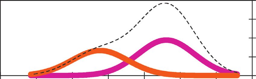
could be resolved easily. implemented. It is easy to see that the model number 3 gives a

Complexity 3

 Open
 12000
 10000
 8000

 Open
 6000
 4000
 2000
 0

 10/31/2021

 6/18/2020

 2/4/2019

 9/22/2017

 5/10/2016

 12/27/2014

 8/14/2013

 4/1/2012
 Date
 Figure 1: The series for the daily closing price index over the period of 1/1/2013 to 16/8/2020.

 Table 1: The descriptive statistics for the daily closing price index over the period of 1/1/2013 to 16/8/2020.
 Summary statistics
 Obs. without missing
Std. Deviation Mean Maximum Minimum Obs. with missing data Observations Variable
 data
 The daily closing price
1126.780 7866.965 11149.360 5416.470 1899 0 1899
 index

 Table 2: Selection criterion is Bayesian information criterion.
 Evolution of the BIC for each model
5 4 3 2 The daily closing price index over
−32040.623 −32025.525 −32010.427 −32107.323 E

 Table 3: The mean by the three components.
Means by class
3 2 1 Class
9232.995 7385.067 7385.066 Mean (open)

Table 4: Selection criterion for selection model. The NEC criterion is more than one which indicates that there is no clustering structure in
the data.
Selection criterion for the selected model
DF Entropy NEC Log-likelihood ICL AIC BIC
6.000 1424.349 25.436 −15982.566 −34859.124 −31977.132 −32010.427

high figure of mean, where model numbers 1 and 2 are closer to MAP classification
 3.5
7385, though the variances are similar in the three models. 3
 2.5
 Classes

 In contrast, the selection criterion can be used to find the
 2
class in the data. It shows that there is more than one 1.5
clustering in this data, where the method gives 25.436. This 1
means that two or three groups can be given (see Table 4). 0.5
 10416.27 9416.27 8416.27 7416.27 6416.27 5416.27
 Figure 2 shows that there are two clusters: the red line
 Open
shows first groups and the green shows the other. This means
that two groups of companies can be gathered together. Figure 2: The MAP classification shows that there is no assignment
More precisely, from the data there are one group going to classes 2.
down and the other going up. It is not easy to find this
information from the data directly. It can be seen that the proposed method gives curve close
 The plots of three model can be found in Figure 3, where to the empirical components. This means that the proposed
the mixed model gives the larger maximum likelihood than method gives excellent results, even compared to various
the other models “1, 2.” models, see Figures 4 and 5.

4 Complexity

 Fitted model mean of the daily closing price index over the study period is
 0.0004
 7866.965. The decline of the daily closing price index in KSA,
 0.0003 which occurred last year, might have been due to COVID-19

 Density
 0.0002 pandemic. The EM algorithm converged in 124 iterations;
 0.0001 according to Bayesian information criterion, the best mix-
 0 ture model is the equal variance with three components (see
 12000 11000 10000 9000 8000 7000 6000 5000 Table 2). The proportions of the three ingredients are varied
 x between 0.261 and 0.370 (see Table 5). The mean of the three
 1 3
 components is run between 9232.995 and 7385.066 (see
 2 Mixture Table 3). The variance of the four ingredients is 610676.444
 (see Table 6). Finally, we must point out that implementing
 Figure 3: The mixture model. such a mechanism to predict the daily closing price index in
 the KSA is beneficial.
 Cumulative distribution function
 1 Data Availability

 distribution
 Cumulative

 function
 0.5
 No data were used to support the findings of this study.
 0
12000 11000 10000 9000 8000 7000 6000 5000
 Date
 Conflicts of Interest
 Empirical CDF The authors declare that there are no conflicts of interest
 Estimated CDF related to this article.
Figure 4: The mixture model. It is clear that the estimated CDF is
very close to empirical CDF, which confirms the accuracy of the Acknowledgments
estimation.
 This work was supported by Taif University Researchers
 Supporting Project (no. TURSP2020/279), Taif University,
 Q-Q plot Taif, Saudi Arabia.
 12000
 Quantiles from

 11000
 References
 the sample

 10000
 9000
 8000
 7000 [1] G. Hu and J. Geng, “Heterogeneity learning for SIRS model:
 6000 an application to the COVID-19,” 2020, http://arxiv.org/abs/
 5000 2007.08047v1.
12000 11000 10000 9000 8000 7000 6000 5000
 [2] M. Qiu and Y. Song, “Predicting the direction of stock market
 Quantiles of the estimated mixture density
 index movement using an optimized artificial neural network
 Figure 5: The quintiles of the estimated mixture density. model,” PLoS ONE, vol. 11, 2016.
 [3] D. Gholamiangonabadi, S. D. Mohseni Taheri,
 A. Mohammadi, and M. B. Menhaj, Eds., in Proceedings of the
 Table 5: The proportions of three components. 2014 5th Conference on Thermal Power Plants, pp. 75–
 Proportions 82pp. 75–, Tehran, Iran, June 2014.
 [4] M. A. I. Khan, “Financial volatility forecasting by nonlinear
3 2 1 Class support vector machine heterogeneous autoregressive model:
0.261 0.370 0.370 Proportions evidence from Nikkei 225 stock index,” International Journal
 of Finance & Economics, vol. 3, no. 4, pp. 138–150, 2014.
 [5] Z. Wang, D.-W. Zhao, L. Wang, G.-Q. Sun, and Z. Jin,
 Table 6: The variance by the three components.
 “Immunity of multiplex networks via acquaintance vaccina-
 Variance by class tion,” EPL (Europhysics Letters), vol. 112, no. 4,
3 2 1 Class pp. 48002–48007, 2015.
610676.444 610676.444 610676.444 Variance [6] Z. Wang, M. A. Andrews, Z.-X. Wu, L. Wang, and
 C. T. Bauch, “Coupled disease-behavior dynamics on complex
 networks: a review,” Physics of Life Reviews, vol. 15, pp. 1–29,
 Article ID 2621171, 2015.
4. Conclusion [7] M. Qiu, Y. Song, and F. Akagi, “Application of artificial neural
 network for the prediction of stock market returns: the case of
This paper used the Gaussian mixtures model to classify the the Japanese stock market,” Chaos, Solitons & Fractals, vol. 85,
daily closing price index over 1/1/2013 to 16/8/2020 in KSA pp. 1–7, 2016.
and describe the problem of predicting the daily closing [8] T. Fischer and C. Krauss, “Deep learning with long short-term
price index in KSA which represents a huge problem. The memory networks for financial market predictions,” European

Complexity 5

 Journal of Operational Research, vol. 270, no. 2, pp. 654–669,
 2018.
 [9] http://file:///C:/Users/DELL/Downloads/Llisting-Guide-2019
 %20(1).pdf.
[10] https://stephens999.github.io/fiveMinuteStats/intro_to_em.
 html#mle_of_Gaussian_mixture_model.
[11] Z. Yao, B. Zhao, L. Qin, Y. Jiang, B. Ran, and Bo Peng, “An
 efficient heterogeneous platoon dispersion model for real-
 time traffic signal control,” Physica A: Statistical Mechanics
 and Its Applications, vol. 539, 2020.
[12] https://www.tadawul.com.sa/wps/portal/tadawul/home/.