Wealth Distribution and Retirement Preparation Among Early Savers

No. 20-4

 Wealth Distribution and Retirement Preparation
 Among Early Savers
 Lindsay Jacobs, Elizabeth Llanes, Kevin Moore,
 Jeffrey Thompson, and Alice Henriques Volz

Abstract:
This paper develops a new combined-wealth measure by augmenting data on net worth
from the Survey of Consumer Finances with estimates of defined benefit (DB) pension
and expected Social Security wealth. We use this concept to explore retirement
preparation among two groups of households in pre-retirement years (aged 40 through
49 and 50 through 59), and to explore the concentration of wealth. We find evidence of
moderate, but rising, shortfalls in retirement preparation. We also show that including
DB pension and Social Security wealth results in markedly lower measures of wealth
concentration, and it slightly moderates trends toward a higher concentration over time.

JEL Classifications: D31, D63, H55, I32
Keywords: retirement adequacy, wealth inequality, Social Security

Linday Jacobs is an assistant professor at the University of Wisconsin’s La Follette School of Public Affairs; her email
is lpjacobs@lafollette.wisc.edu. Elizabeth Llanes is a PhD student in the University of Wisconsin’s Department of
Economics; her email is llanes@wisc.edu. Kevin Moore is the chief of the Microeconomics Survey Section in the
Research and Statistics department of the Board of Governors of the Federal Reserve System; his email is
kevin.b.moore@frb.gov. Jeffrey Thompson is a vice president and economist in the research department of the Federal
Reserve Bank of Boston; his email is jeffrey.thompson@bos.frb. Alice Henriques Volz is a principal economist in the
Microeconomics Survey Section in the Research and Statistics department of the Board of Governors; her email is
alice.h.volz@frb.gov.

The authors thank John Sabelhaus; seminar attendees at NTA, George Mason University, the Congressional Budget
Office, and the Federal Committee on Statistical Methodology for useful comments and feedback; and Melissa Gentry
for excellent research assistance.

This paper presents preliminary analysis and results intended to stimulate discussion and critical comment. The
analysis and conclusions set forth are those of the authors and do not indicate concurrence by other members of the
research staff of the Board of Governors, the Federal Reserve Bank of Boston, or the University of Wisconsin.

This paper, which may be revised, is available on the website of the Federal Reserve Bank of Boston at
https://www.bostonfed.org/publications/research-department-working-paper.aspx.

This version: February 2020 https://doi.org/10.29412/res.wp.2020.04

The wealth that households accumulate during their working years—through pensions, housing

equity, and other types of assets—is crucial in providing support to sustain them in retirement.

There is a large literature evaluating the adequacy of retirement resources among retirees and

households transitioning into retirement, and there is also a growing literature using wealth data

to explore inequality in the distribution of economic resources—beyond the more traditional

emphasis on income and consumption. This paper uses the Federal Reserve Board’s triennial

Survey of Consumer Finances (SCF) to contribute to each of these areas of research.

The SCF is the only household survey that provides adequate coverage of high-net-worth

households in the United States. The wealth concept in the survey, market wealth, is incomplete,

however, particularly when evaluating retirement resources. Importantly, household wealth in

the SCF does not adequately reflect the asset value of defined benefit (DB) pensions. Further, it

does not include the value of the future Social Security benefits that workers will accrue over

their lifetime. These additional forms of wealth are important resources to retirees, but they also

impact decisions leading up to retirement. Crucially, they disproportionately benefit households

below the top portion of the wealth distribution. Therefore, they are vital for understanding the

full distribution of wealth and for assessing the adequacy of savings of workers who will be

transitioning into retirement in the future.

We develop an expanded definition of household wealth (“combined” wealth). First, we augment

the asset and debt information collected in the SCF with estimates of the asset value of both

traditional DB pensions and expected Social Security benefits. Second, we project SCF net worth

following income-wealth-specific growth patterns observed in the survey, creating a wealth

measure with timing that is in line with the estimation of expected Social Security wealth at the

 2

early eligibility age. We also project forward our DB estimates to reflect expected accumulation

of benefits from one’s current job.

We first use this combined-wealth concept to evaluate the resources of households approaching

retirement age. Most of the retirement-adequacy literature focuses on recently retired or about-

to-retire workers. We evaluate preparation among households whose heads are in their 50s,

similarly to existing studies, but also among a cohort of “early savers,” households whose heads

are in their 40s. Consistent with much of the literature, we find that expected retirement income

is adequate for most households, but leaves a substantial—and growing—number at risk

financially during their retirement years.1

We next use the expanded-resource concept to calculate levels and changes in the distribution of

wealth over time. Some of the existing research exploring the distribution of wealth uses data

that do not include households at the very top of the wealth distribution, and most of the data do

not reflect either the implied asset value of DB pensions or Social Security.2 Incorporating the

asset value of expected retirement benefits, particularly Social Security, has a dramatic

equalizing effect on the distribution of wealth. For example, among households with heads aged

40 to 49, the top 5 percent’s share of wealth excluding retirement plans (defined-benefit [DB],

defined-contribution [DC]) and Social Security is 53 percent. Once these assets are included, the

top 5 percent’s wealth share falls to 38 percent. There is also a slight moderation in the trend

toward greater inequality once we incorporate all forms of retirement wealth.

1
 Using administrative data, both Bee and Mitchell (2017) and Beshears et al. (2019) find that income in
retirement, on average, has not fallen dramatically over the past 10 to 20 years. Beshears et al. (2019) do show
deterioration for those with below-median income.
2
 Wolff (2014, 2015) is the primary exception here, as he also uses the SCF and predicts earnings histories. His
focus is primarily on the Gini coefficient and broad inequality trends, not specifically top-end concentration. There
are also a several methodological differences between this paper and Wolff’s papers.

 3

In the remainder of this paper, we:

  briefly review the retirement-adequacy and wealth-inequality literatures, drawing

 attention to the contributions that we make in this paper

  describe the primary data we use in this analysis—the SCF

  detail the methods and additional data sources we use in estimating household-level

 earnings histories, which are used to calculate expected Social Security benefits and age-

 forward the private wealth measures to the point of retirement

  present our findings, both for retirement preparation and for the distribution of wealth

2. Literature Review

Retirement-income adequacy and wealth concentration have each generated an extensive

literature. With a focus on identifying this paper’s contributions, we provide a very brief

overview of these two literatures.

2A. Retirement Adequacy

The extensive literature evaluating the adequacy of income for current and future retirees has

been spurred by dramatic changes in the demographics of an aging country and equally dramatic

changes in our retirement system, which has transformed from a primarily defined-benefit (DB)

pension system to an overwhelming defined-contribution (DC) system in just a few decades. The

now-ubiquitous 401(k) plan was introduced into law in 1978. As of the late 1980s, traditional

DB pensions were still the typical plan for households with heads aged 40 to 59. In 1989, 25

percent of these households were covered by a traditional defined benefit pension only, 17

percent by a DC plan only, and 18 percent by both types of plans (Figure 1). By 2016, 7 percent

had only a DB plan, 8 percent had both types of plans, and 37 percent relied on DC plans

 4

exclusively for their work-based pension. This transformation of the pension system has made

benefits more flexible and portable—virtues appreciated by many workers. But, it has also

shifted risk and decision-making from employers to workers, fueling considerable anxiety about

retirement preparation and retirement income being exposed to the volatility of investment

returns.

As this transformation of the pension system has unfolded, numerous researchers have sought to

understand the consequences for the adequacy of retirement income for older Americans. On the

central question of the status of the adequacy of retirement income, the literature is divided.

Some papers identify large shortfalls in the adequacy of retirement savings (Bernheim 1992;

Munnell, Webb, and Delorme 2006; Munnell, Rutledge, and Webb 2014; Munnell, Hou, and

Sanzenbacher 2018; Haveman et al. 2006; Munnell, Orlova, and Webb 2013). Others conclude

that household financial preparation for retirement is in much better shape, and any shortfalls are

largely concentrated among specific, more vulnerable groups, such as single retirees (Engen,

Gale, and Uccello 1999; Sholz, Seshadri, and Khitatrakun 2006; Love, Smith, and McNair

2008).

Defining Adequacy

One of the methodological factors that differentiate these—and other—studies from each other is

the way they define “adequacy.” Adequacy is typically determined by comparing anticipated

household income in retirement with pre-retirement income. Replacement rates are deemed

“adequate” if they provide a smoothed level of consumption across a household’s working life

into retirement, with a potential step-down adjustment at the point of retirement.3 Another

3
 See Biggs and Springstead (2008) for a discussion of alternative standards of adequacy of replacement rates.

 5

approach to defining adequacy assumes declining levels of consumption over the retirement

period, based on models in which households smooth the marginal utility of consumption over

the life cycle; these models use assumptions on preference parameters and changes in

consumption when children leave home (Sholz, Seshadri, and Khitatrakun 2006; Engen, Gale,

and Uccello 1999).

The differences between these first two approaches to defining adequacy go a long way toward

reconciling the competing pessimistic and more optimistic findings from the research on

retirement adequacy. When Sholz, Seshadri, and Khitatrakun (2006) assume a more standard

life-cycle rule that defines annual retirement consumption as a function of lifetime resources,

they find that 49 percent of households have inadequate savings, compared with only 16 percent

under their declining rate optimized path of consumption. Similarly, when Munnell, Rutledge,

and Webb (2014) adjust the adequacy rules in the National Retirement Risk Index (NRRI) to

incorporate the optimal rates of asset drawdown implied in Sholz, Seshadri, and Khitatrakun

(2006), the share of households (heads aged 51 to 61) with inadequate retirement resources falls

from 35 percent to 24 percent. When they also incorporate the assumption that Sholz, Seshadri,

and Khitatrakun (2006) use regarding the decline in consumption after children leave the home,

the share of households with inadequate savings falls further to 11.5 percent.

A third approach uses an external benchmark to indicate target levels of consumption in

retirement (Wolff 2002; Haveman et al. 2006; Love, Smith, and McNair 2008). One implication

of the replacement-rate and smoothed-consumption approaches to defining “adequacy” is that,

because they are determined relative to the household’s own income history, poor households

that are able to maintain the same poverty-level consumption in retirement are considered to

 6

have “adequate” resources. Households with much higher absolute standards of living might be

considered to have inadequate resources.

Most studies that employ external benchmarks to assess adequacy use the official poverty

thresholds, which vary over time and by household composition. Use of the poverty thresholds,

however, has been criticized because, detractors argue, they are too low ($14,507 for an elderly

couple in 2016) to represent a meaningful standard of well-being for retirees. Gould and Cooper

(2013) use the Supplemental Poverty Measure (SPM), which reflects health-care costs and

regional differences in cost of living. Mutchler, Li, and Xu (2016) develop an “Elder Index,”

which is based explicitly on costs faced by seniors and varies by household composition,

homeownership status, and regional cost differences. These alternative benchmarks are much

higher than the poverty threshold, thus resulting in larger shares of current and future retirees

falling below “adequate” levels of retirement income. Hurd and Rohwedder (2011) use observed

consumption paths over retirement from panel data (the Health and Retirement Study) as a

benchmark, identifying adequacy among recent retirees as sufficient income to afford retirement

consumption and still be able to leave a bequest. Although the official poverty thresholds are

much lower than these alternative benchmarks, they have been produced consistently for decades

and can be used to explore changes in adequacy over time.

This study does not take a stand on the optimal definition of adequacy and instead presents a

variety of measures that allows one to piece together an overall picture of adequacy.

Measurement of Retirement Income & Assets

Most research on retirement income adequacy uses data from the Health and Retirement Study

(HRS). The HRS is a high-quality household survey of older Americans that includes a battery of

 7

questions on household income and resources. In recent years, researchers have been able to link

the HRS to individual Social Security earnings histories and to employer-specific pension plans.

Studies using the HRS either explore adequacy among current retirees (Hurd and Rohwedder

2011; Moore and Mitchell 1997) or use the survey’s self-reported expected pension and benefits

income data to explore income adequacy for those about to retire (Engen, Gale, and Uccello

1999; Love, Smith, and McNair 2008).

The HRS offers many advantages to researchers in this field, but it has some limitations as well.

Due to the survey design, the HRS cannot tell us anything about the savings or anticipated

retirement adequacy among younger workers. Several studies using the HRS evaluate adequacy

among workers as young as 51 years old (Munnell, Orlova, and Webb 2013; Gustman and

Steinmeier 1999; Scholz, Seshardi, and Khitatrakun 2006). Ideally, however, retirement

preparation starts much earlier in the life cycle. Also, because it does not include high-net-worth

households, the HRS cannot be used to fully evaluate the implications of Social Security on

wealth concentration.4

Several other studies explore retirement adequacy using the Survey of Consumer Finances

(SCF). Because the SCF samples the entire age distribution, these studies are able to look at

retirement income among younger cohorts of savers. Kennickell and Sunden (1997) use the age-

earnings profile from one year of Current Population Survey (CPS) data to predict earnings

histories of households whose heads are younger than 65 years old.5 Wolff (2002, 2007, 2015)

predicts earnings histories within the SCF using an in-sample estimation of future earnings based

4
 While the ability to match to Social Security earnings is extremely useful, not all respondents agree to the match,
and researchers need to estimate earnings for the missing records. There is some evidence of bias introduced by the
selection of respondents who agree to the match (Bricker and Engelhardt 2014).
5
 Given the early time period considered, Kennickell and Sunden (1997) show an equalizing effect on wealth
distribution of DB and Social Security wealth, but not of DC wealth.

 8

on a simple human capital earnings regression in conjunction with respondent-provided current-

and past-job information. These predicted retirement incomes are used to evaluate adequacy in

several years of the SCF for cohorts that are younger (47 to 64 years olds [Wolff 2002, 2007]

and 40 to 55 year olds [Wolff 2007]) than those evaluated using the HRS.

The National Retirement Risk Index (NRRI), developed by the Center for Retirement Research,

also uses the SCF to evaluate retirement adequacy. The NRRI imputes earnings histories into the

SCF through a statistical match with the linked HRS/Social Security earnings data. The NRRI

calculates adequacy across the full age distribution. Since the HRS includes only workers in their

50s and older, several additional assumptions are needed to predict earnings histories and future

earnings for younger workers.

All the above SCF studies use the self-reported DB pension responses in the SCF and rely on

out-of-sample data to predict earnings histories for the purpose of calculating future Social

Security benefits. This paper aims to improve on both of these solutions to measurement

challenges in order to enhance our understanding of retirement preparation over the life cycle

and across the distribution of household resources.

A final related area of the literature focuses on the adequacy of retirement income for individuals

who have recently retired. Brady et al. (2017), for example, find that most individuals maintain a

high replacement rate of pre-retirement income after they retire, but the authors acknowledge

that there is variability across the income distribution.6 This strand of the literature uses panel tax

data to follow the changes in income in pre-retirement and retirement years and is more focused

on the contribution of the different types of retirement income (such as Social Security and

6
 Beshears et al (2019) come to a similar conclusion.

 9

pensions) to overall retirement income. Due to the research design and data source, these studies

focus on individuals near retirement age and cannot examine the accumulation of assets before

retirement.

2B. Wealth Distribution

That wealth—particularly financial assets—is highly concentrated at the top of the distribution

has long been acknowledged and, in fact, is the motivation for the unique sampling strategy

employed in the Survey of Consumer Finances (SCF). Results from the 1989 SCF indicate that

the top 1 percent of households held 16 percent of all income but 30 percent of net worth

(Bricker at al. 2016). Most research exploring the distribution of wealth in the United States

relies on the SCF (Bricker et al. 2016; Keister and Moller 2000; Wolff 1995; Kennickell 2006).

Some wealth distribution research uses the Panel Study of Income Dynamics (PSID), which also

includes questions on assets and debt (Quadrini 1999; Banks, Blundell, and Smith 2003; Fisher

et al. 2016). These studies yield lower estimates of wealth concentration because the PSID does

not adequately sample high-wealth households, and it does not ask about some asset types that

are disproportionately held by the wealthy (Juster, Smith, and Stafford 1999; Pfeffer et al. 2016).

The top 5 percent’s wealth share for 1989 was 47 percent in the PSID, but 57 percent in the SCF

(Wolff 2007).

Wealth is highly concentrated, and accurate measurement of its concentration is highly

dependent on the use of data that include high-wealth households. The extent to which the

concentration of wealth has risen over time, however, is in dispute. Analysis of net worth

reported in the SCF suggests top-wealth shares have increased somewhat, with the top 1

percent’s share climbing to 38 percent by 2016 (Bricker et al. 2017). In an alternative approach,

Saez and Zucman (2016) use a capitalization model to predict wealth based on flows of capital

 10

income reported on federal income tax forms and rates of return estimated from the Federal

Reserve Board’s Financial Accounts of the United States and other macrodata sources. They find

that wealth predicted from tax returns rises in much the same way as reported wealth does—with

the top 1 percent’s share climbing from 28 percent in 1989 to 39 percent in 2016.

Each of these studies improves our understanding of trends in the distribution of wealth, but

neither uses a wealth concept that includes the implied asset value of Social Security benefits.

Devlin-Foltz, Henriques, and Sabelhaus (2016) show that including improved measures of DB

pension wealth results in somewhat lower measures of wealth concentration in the SCF, and we

build directly on that work. The absence of Social Security from the discussion of wealth

concentration is troubling for several reasons. Social Security benefits represent the single-

largest source of retirement income for more than 60 percent of retired households (Social

Security Administration 2016). Because the accumulation of wealth to finance retirement is the

dominant reason for saving, and Social Security may “crowd out” private savings or is the

primary savings mechanism for many lower-income households, discussions of wealth

distribution, especially in the context of economic policy, that do not include the value of Social

Security are limited at best and potentially misleading.

3. Data and Methods

For the purposes of improving the measurement of wealth concentration and extending the

research on retirement income adequacy to a younger cohort of households, we use the Survey of

Consumer Finances (SCF) to develop an expanded measure of wealth that incorporates estimates

of DB wealth as well as the asset value of Social Security among the 40- to 59-year-old

population. We directly incorporate the work of Sabelhaus and Volz (2019), who impute the

value of DB wealth to current workers in the SCF using labor market and pension plan

 11

characteristics in the survey along with high-quality external data on DB plan assets. In this

section, we discuss the SCF and the methods we use in (1) estimating earnings histories of

survey respondents, (2) calculating future Social Security benefits, and (3) aging-forward net

worth reported in the SCF to the point of retirement.

Our research represents an improvement on work by others using the SCF to develop broader

wealth measures for the purpose of assessing retirement adequacy (NRRI studies by Munnell et

al. various years) or the distribution of wealth (Wolff various years). Both Wolff and Munnell et

al. rely solely on self-reported information on pensions in the SCF to estimate DB wealth for

future retirees, which results in levels of predicted pension wealth that are inconsistent with

economy-wide pension assets.7 Following Sabelhaus and Volz (2019), we instead combine

aggregate data on plan assets with the SCF survey data to estimate DB wealth of current

workers. (See Section 3B below and Appendix A for additional details.) In calculating Social

Security wealth of current workers, Wolff estimates in-sample human capital equations to predict

future covered earnings, and Munnell at al. statistically match SCF workers with a standardized

earnings trajectory based on linked HRS-Social Security earnings records. The static age-

earnings profiles embodied in Wolff’s approach fail to capture how workers’ earnings evolve

over time, an element we incorporate in our analysis using cohort earnings trajectories. (See

Section 3C below for details on our approach.)

3A. The SCF

7
 Wolff (various years) combines self-reported future pension coverage with an estimate of future earnings. The
NRRI studies by Munnell et al. also make assumptions about declining generosity across cohorts and about future
coverage for younger cohorts without DB pensions.

 12

The primary data source we use are the 10 waves of the triennial Survey of Consumer Finances

(SCF) conducted from 1989 through 2016. Several features of the SCF make it appropriate for

exploring retirement-income adequacy and the distribution of wealth. The survey collects

detailed information about households’ financial assets and liabilities, and has employed a

consistent design and sample frame since 1989. As a survey of household finances and wealth,

the SCF includes assets that are broadly shared across the population (bank savings accounts) as

well as assets that are held more narrowly and are concentrated in the tails of the distribution

(direct ownership of bonds).

To support estimates of a variety of financial characteristics as well as the overall distribution of

wealth, the survey employs a dual-frame sample design. A national area-probability (AP) sample

provides good coverage of widely held assets and debts. The AP sample selects household units

with equal probability from primary sampling units that are chosen through a multistage

procedure, which includes stratification by a variety of characteristics. Due to the concentration

of assets and non-random survey response rates by wealth, the SCF also employs a list sample

that is developed from statistical records derived from tax returns under an agreement with the

IRS’s Statistics of Income (SOI) program.8 This list sample consists primarily of households

with a high probability of having high net worth.9 The SCF combines the observations from the

AP and list samples through weighting, and the weighting design adjusts the samples separately

using the information available for each one. The final weights are adjusted so that the combined

8
 See Bricker et al (2014) and Bricker et al (2017) for recent discussions of the sampling strategy, the list sample,
and the weights used in the SCF. See Wilson and Smith (1983) and Internal Revenue Service (1992) for a
description of the SOI file. The file used for each survey largely contains data from tax returns filed for the tax year
two years before the year the survey takes place.
9
 For reasons related to cost control on the survey, the geographic distribution of the list sample is constrained to that
of the area-probability sample.

 13

sample is nationally representative of the population and assets.10 These weights are used in all

calculations.

The primary purpose of the SCF is to collect information about household balance sheets.

Among the items measured in the SCF is the value of all financial and nonfinancial assets,

including residential and non-residential real estate and privately held businesses, reported by the

respondent at the time of the interview.11 Questions on household debt reflect all types of debt,

including credit cards, mortgage debt, student loans, business debts, and other miscellaneous

forms of debt.12

3B. Defined Benefit Pension and Social Security Wealth

One shortcoming of the SCF, with regard to measuring both retirement-income adequacy and

wealth concentration, is the omission of current asset values of future DB pension payments and

Social Security benefits. Respondents enrolled in DB pension plans are asked questions about

expected future benefits. Many workers, particularly those further from retirement age, may have

limited knowledge about their plans or future benefits, and so the information collected from

these questions is not necessarily an accurate reflection of what the respondents will actually

receive (Starr-McCluer and Sunden 1999).

10
 The SCF weights were revised in 1998 to incorporate home ownership rates by race (Kennickell 1999). Weights
for earlier years were updated to reflect the revised methodology.
11
 Assets do not include—and the SCF does not collect—information on the value of DB pensions or the implied
annuity value of future or current Social Security benefits of respondents.
12
 The unit of analysis in the SCF is the “primary economic unit” (PEU), which refers to a financially dependent and
related (by blood, marriage, or unmarried partners) group living together. This concept is distinct from both the
household and family units employed by the US Census Bureau, but is conceptually closer to the latter, and
throughout this paper PEUs are referred to as “families.” Single individuals living alone are included and considered
simply a “family” of one.

 14

Instead of relying fully on the expected future benefit responses provided by DB plan

participants, we rely on the estimated DB pension wealth for SCF households developed by

Devlin-Foltz, Henriques, and Sabelhaus (2016) and Sabelhaus and Volz (2019). Their approach

assigns aggregate household sector DB assets from the Financial Accounts of the United States

(FA) to both current and future beneficiaries using survey information on benefits currently

received for those receiving payments, reported future payments for those with coverage from a

past job, and wages and years in the plan for those not yet receiving benefits. The authors

combine the survey information with real discount rates that fluctuate over time, cohort life

tables, differential mortality estimates, and the assumption that current beneficiaries have first

claim to DB plan assets.13 Devlin-Foltz, Henriques, and Sabelhaus (2016) find that inclusion of

the implied assets from future pension benefits modestly reduces inequality in the distribution of

wealth, but they do not include implied wealth from future Social Security benefits in their

discussion of wealth distribution. To develop estimates of future Social Security benefits, and

their implied asset value, we first need to estimate earnings histories (and projections) for

respondents and their spouses in the SCF.

3C. Methodology for Estimating Earnings Profiles in the SCF Using CPS Cohorts

To construct a full earnings history and projections of future earning for SCF respondents, we

apply the growth in earnings over one’s working life implied by the shape of the Current

Population Survey (CPS) earnings estimates for individuals who are most similar to the SCF

respondents based on birth year, occupation, education level, and sex.

13
 See Appendix A for more details on DB wealth estimation.

 15

From the 1989–2016 SCF data, we take respondents aged 40 to 59 (with spouses aged 30 to 65)

at the time of the interview and use (1) information reported on current occupation, earnings, and

tenure; (2) any retrospective information on occupation, earnings, or tenure; and (3) information

reported on future work expectations. For each respondent and spouse, we estimate a full history

of past and future earnings using regression analysis described below that rely on CPS data from

1964 through 2016.

Individuals are categorized into types by 21 possible birth-year cohorts (three-year cohorts from

the 1924–1926 period through the 1984–1986 period), three education levels (less than high

school, high school or equivalent, some college/degree), and five broad occupation categories

([1] management, professional, and related; [2] service; [3] sales and office; [4] construction,

maintenance, production, transportation; and [5] self-employed from all occupations).

For some ages, we broaden the categories, defining an individual by education-occupation types

(for men and women separately) instead of age when that person’s birth-year cohort is not

observed in the CPS at those ages. For instance, the youngest person whose earnings profile we

want to estimate was born in 1986 and was 30 years old at the time of the 2016 SCF interview.

The estimates will be based on earnings of those born in the 1984–1986 period who were as old

as 32 in the 2016 CPS. To forecast earnings growth after age 32, we use coefficient estimates

from the education-occupation model. Similarly, for the oldest birth year in the earliest (1989)

SCF, 1924, we use the education-occupation model coefficients to fill in a person’s earnings at

each age before 1964. Those born between 1942 and 1951 are fully covered by the CPS.

For each person type , we estimate the following regression on log income in the CPS:

 ln( ) = 0 + 1 + 2 2 + 3 3 + 4 4 + 

 16

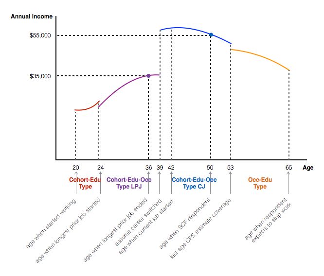
and back out a person’s individual effect, 0 , at the time of the SCF survey

 0 = ln( ) − 1 + 2 2 + 3 3 + 4 4 + .

The individual effect in any year is a weighted average of the individual and group constants, 0 
 
and 0 , respectively, where we place more weight on the group average constant as we estimate

periods further out from the reported income in the SCF. Specifically, the constant at time t is
 
 , = 0 + (1 − ) 0 , where we set = 0.85.

To predict income, we then apply , , 1 , 2 , 3 , 4 , for all ages for each

individual.14 Anyone who reports a longest previous occupation type that is different from their

current occupation will have different coefficients applied to the relevant years.

As an example, suppose we have a 2013 SCF respondent who is 50 years old at the time of the

survey and reports current full-time earnings of $55,000 in his current job of eight years. His

reported longest previous job, which lasted 12 years, was in a different occupation and ended 14

years ago with his earning $35,000. He reports having worked full-time every year since age 20

and expects to stop working at age 65. The earnings history and earnings projection for this

individual would look something like what is shown in Figure 2.

We assume when estimating an individual’s future income that they will work until their

expected retirement age, reported in the SCF, which will, of course, not be the case for everyone.

The CPS income estimated for a person’s type will account for relatively short periods of

unemployment, as it includes total income for those who were not employed for the entire

14
 There are 786 possible types: 630 of the more specific cohort-occupation-education-sex combinations, 126
cohort-education-sex combinations (applied when occupation is unclear), and 30 occupation-education-sex
combinations (applied when estimating earnings if outside the ages the birth-year cohort is observed in the CPS or
when some information is missing).

 17

previous year. However, with these measures, we will not be able to capture losses in income

due to long-term unemployment, unanticipated early or partial retirement, or permanent labor

force exit through disability, all of which could be modeled through shocks in future studies.

Our current SCF lifetime income estimates match the CPS well at younger ages, but they are

relatively high at older ages (see Appendix Figures 1A and 1B for comparisons for two

different birth-year cohorts of men). We attribute this difference primarily to lower income from

partial retirement being captured in the CPS but not in the SCF retirement expectations and, to a

lesser extent, to the differences in the SCF and CPS sample frames.

3D. Details of Social Security Benefits Calculations

Armed with an earnings profile for each individual from ages 20 through 61, one can apply

Social Security benefit calculations for each household. First, nominal earnings are indexed to

age 60, and the highest 35 are used to calculate each individual’s averaged indexed monthly

earnings (AIME). The AIME is transformed into a monthly payment using the primary insurance

amount (PIA) formula and the cohort-specific actuarial adjustment. We assume all individuals

begin receiving Social Security benefits at age 62, which provides a lower bound for total

household Social Security wealth (SSW). Additional benefits are discounted to the survey year

using a 3 percent real discount factor and survival rates that vary by cohort, marital status, race,

and education (relying on cohort life tables from the Social Security Administration and

differential mortality estimates from the Congressional Budget Office).

Wives (using the term generically for clarity but referring more broadly to secondary earners) are

entitled to their own benefits (if eligible) but also spousal and survivor benefits. We assign

spousal benefits to the household if they are expected to be greater than the wife’s worker

 18

benefits at age 62. If the duration of the current marriages is less than 10 years when the wife

reaches 62, she does not receive spousal or survivor benefits.15

The measure of SSW used is net of expected future employee contributions. Thus, for every year

(after the survey), we calculate expected tax payments of 6.2 percent and subtract the present

value of all future contributions from the gross SSW measure calculated (as detailed above).

3E. Creating the Combined-Wealth Measure

The combined-wealth measure that we analyze below incorporates (1) the implied wealth from

Social Security benefits net of contributions and including projected earnings from future work

up until the time of retirement, (2) wealth from DB pensions projected to the expected job end

date, and (3) projected future wealth from all assets and debt measured directly in the survey.

To be consistent with the estimates of future Social Security wealth (which reflect expected

benefits at age 62, not just those that had been accrued as of the interview date), we project the

anticipated value of the SCF sample net worth, not including DB wealth, to age 62 (part [3]

above). These projections are based on in-sample estimates of the growth paths of wealth from

age 40 to 62 using all 10 SCF cross-sections (1989 through 2016). We categorize each household

into one of nine groups based on its location in the distribution of “usual” income—an income

concept included in the SCF that smooths away transitory fluctuations16—and current wealth

among households in each survey.17 We then estimate age-wealth profiles separately for each of

15
 The SCF does not collect information about length of previous marriages, thus some individuals with more than
one marriage will not be accurately assigned dependent benefits from a former spouse.
16
 See Ackerman and Sabelhaus (2012) for further discussion.
17
 The categories are all combinations of the bottom 40 percent, next 40 percent, and top 20 percent for both income
and wealth. Households were divided into these categories to estimate the growth in wealth for households showing
the most similar wealth-accumulating behavior within their income group. The categories were kept relatively
broad, however, to capture the group in which a household would be likely to remain over the ages of 40 to 62. For
the years 1995 through 2016, usual income is used to rank households. For the 1989 and 1992 surveys, which
predate the usual income question, we use current income.

 19

the nine categories, pooling all surveys, and apply the growth rates from these profiles to project

households’ survey wealth to age 62. Separate profiles are estimated for housing wealth, defined

contribution (DC) pension wealth, and all other forms of wealth measured in the SCF. The

implied annual growth rates of combined wealth for each of the nine income-wealth cohorts over

the 40–62 age span are higher for the lowest wealth cohorts (Appendix Figure 2). Among

middle- and high-wealth households, the growth rate of wealth is highest for those in the top 20

percent of both wealth and usual income. Because the annual rate of growth in wealth is higher at

younger ages, and we discount the projected wealth back to the age when we observe households

in the sample, the net effect of the wealth projections is substantially larger for younger

households (Appendix Figure 3).18

We also project DB wealth to an individual’s expected job ending date or age 59, whichever

comes first. This brings DB wealth in line with both SSW and projected DC wealth to

acknowledge that individuals may have many more years of accumulating benefits, and it allows

us to better compare age groups over time. To do so, we back out of the Sabelhaus and Volz

(2019) accrued DB wealth the “generosity factor” implied by the allocation. The generosity

factor reflects a percentage of final wages given as a DB benefit for each year of service one

accumulates. For example, in a plan with a 1 percent generosity factor, an individual with 30

years of service would receive 30 percent of their final wages as a DB benefit. With a generosity

18
 This approach is different from the one taken by Munnell, Rutledge, and Webb (2014) in measuring future wealth.
As a part of constructing the NRRI, Munnell, Rutledge, and Webb (2014) measure, for distinct components of
wealth, wealth-to-income ratios by age in the SCF. They calculate target age-specific savings rates—for 48 different
household types based on income, composition, homeownership status, etc.—that would be required for the
households to achieve a level of wealth where post-retirement consumption is equal to consumption just before
retirement. Making projections for each component separately, as is done to construct the NRRI, will not necessarily
be an improvement for the analyses in this paper. Projections based on a single model of total net worth produced
growth paths similar to those from the current approach of separate projections for housing, retirement, and
remaining wealth. This results from households within a given income-wealth category having relatively similar
compositions of net worth components.

 20

factor, one can project a final DB payment for each individual, given their projected wages.

Expected DB payments then are transformed into present discounted value as of the survey date.

The combined-wealth measure we analyze below combines the net present value of projected

SCF net worth with projected DB wealth and expected future Social Security wealth.

3F. Retirement Preparation Concepts

We use two simple measures of household preparation for retirement. The first is wealth-to-

income ratio. It divides our expanded wealth concept by the current reported household income.

The second is an annuity measure of wealth. We compare the estimated annuity amount with the

poverty level for elderly households, either one- or two-person households depending on the

marital status of the respondent.19 We also calculate the share of the population falling below

various multiples of the poverty threshold. For these two basic measures of retirement income

adequacy, we explore trends over time for both age groups, 40 to 49 and 50 to 59.

4. Results

In this section, we describe the results for both retirement income adequacy and wealth

concentration using our combined-wealth measure. We show results over time for each SCF

cross-section from 1989 through 2016, and for both the 40–49 and 50–59 age groups. We first

show means, medians, and total levels of various wealth categories. Next, we show wealth-to-

income ratios, followed by annuitized poverty measures. Then we calculate wealth-percentile

ratios and concentration measures.

19
 Our annuity calculation is the same as that used by Love, Smith, and McNair (2008). We divide the present value
of our combined-wealth measure (net worth, including DC wealth, plus the net present value of Social Security and
DB pension wealth) by the actuarially fair price of an annuity. The price is the sum of the probabilities of surviving
to advanced age levels for both respondent and, if present, spouse, and it also assumes a 3 percent discount rate.

 21

4A. Retirement Wealth and Combined Wealth

4A.i. Components of Retirement Wealth

The average wealth in defined contribution (DC) plans held by both age groups has followed a

familiar path, rising substantially in the years before the financial crisis, experiencing a period of

stagnation, and then reaching a new peak in the 2016 survey. Among 50- to 59-year-olds, mean

DC balances were $53,000 in 1989, rose to $164,000 by 2007, fell back to $146,000 by 2013,

and rose to a new high of $177,000 by 2016 (Figure 3, right panel). Mean DC balances are

considerably lower for the 40–49 age group, starting at $35,000 in 1989 and reaching $94,000 in

2016 after hitting a plateau of about $80,000 from 2001 through 2013 (Figure 3, left panel). As

DC accounts were not introduced until the late 1970s, it is not surprising that average balances

were low in 1989. The data indicate substantial preparation before age 40, but a considerable

amount of retirement wealth accumulation is also taking place as households move closer to

retirement.

For the 40–49 age group, mean DB wealth started at $90,000 in 1989, peaked in 2007 at

$156,000, and was $148,000 in 2016 (Figure 3). Mean DB wealth for 50- to 59-year-olds was

$278,000 in 2001 and fell across the remaining waves, hitting $206,000 in 2016. Some of the

difference in DB wealth we observe between the two age groups is mechanical; the same future

benefit has to be discounted further back in time for younger ages. In addition, DB coverage is

lower for younger workers, particularly in later years.

Predicted Social Security wealth (SSW) accounts for the largest portion of retirement wealth for

both age groups in almost all years. Mean SSW rose from $127,000 in 1989 to $150,000 in 2016

 22

among 40- to 49-year-olds, and it rose from $189,000 to $238,000 over the same period for 50-

to 59-year-olds. SSW rises along with earnings growth in the working population, and it has

fallen slightly for the older age group since the financial crisis. The broad growth in SSW,

particularly in the 1990s, has come generally from two sources: higher real wages and increased

labor force participation among women.

4A.ii. Combined-Wealth Measures

It is well known that the financial crisis and housing market crash led to large losses of wealth

throughout the economy. The bulk of these losses occurred in assets that are not specifically

identified as forms of retirement saving (Bricker, Moore, and Thompson 2019). “Non-

retirement” wealth here includes housing and other forms of financial and nonfinancial wealth,

and it excludes DC and DB wealth and expected Social Security wealth.

For all comparisons going forward, non-retirement wealth, DC wealth, and housing wealth are

projected to age 62, and for those in a DB plan, DB wealth is projected to the age they expect to

separate from the firm for which they currently work. This puts all wealth measures on equal

footing, allowing for better comparisons across age groups and over time. Due to life-cycle

patterns, those in their 40s are expected (and shown, in Figure 3) to have less wealth

accumulated for retirement. This does not, however, imply that the younger age group is less

prepared for retirement.

The first set of bars in the left and right panels in Figure 4 shows that there is little change in

non-retirement wealth over the full period, save for the short-lived run-up in housing wealth for

the 40–49 age group leading up to the financial crisis; among 50- to 59-year-olds, non-retirement

wealth increased more substantially. The middle set of bars, which combines non-retirement

 23

wealth with private retirement wealth, indicates that when DC and DB pensions are included,

average wealth has increased over time for both age groups, although the growth has been

substantially greater for 50- to 59-year-olds, particularly in 2016 in non-retirement wealth.

A similar pattern of growth in mean wealth persists once we incorporate projected net Social

Security wealth. For 40- to 49-year-olds, mean combined wealth—including non-retirement

wealth, DC and DB pension wealth, and net Social Security wealth—rose from $943,600 in 1989

to $1.2 million in 2007, fell to $962,000 by 2010, and then partially recovered to $1 million by

2016 (Figure 4). Among 50- to 59-year-olds, it rose from $900,000 in 1989 to $1.5 million in

2007, before falling to $1.3 million in 2010, and recovering to almost $1.5 million in 2016.

Compared with the mean values, the median of the distribution of combined wealth rose less

between 1989 and 2007 and fell relatively further after the financial crisis for both age groups

(Table 1). Median combined-wealth levels were lower in 2016 than in 1989. Nearly all of the

decrease in median combined wealth was due to the decline in non-retirement wealth (Table 2).

4A.iii. Combined Wealth across the distribution

The individual components of the combined-wealth measure have very different distributions.

We explore the wealth levels at different points in the distribution in two ways. First, we look at

the distribution for each of the wealth components—non-retirement wealth, DC and DB wealth,

SSW—and combined wealth by age group and year. This highlights the fact that some

components of combined wealth are distributed more equally than others.

Most households have no DB pension wealth, thus the values at the 10th, 25th, and 50th

percentiles of DB pension wealth are zero for both age groups in 2016 (Table 1). Furthermore,

more than one-quarter of households do not have any DC pension wealth. A majority of

 24

households do have a DC plan, but the median of the overall DC wealth distribution was just

$4,200 in 2016 among 40- to 49-year-olds and only $6,400 among 50- to 59-year-olds. Both

non-retirement wealth and Social Security wealth are far more broadly distributed than is either

DB or DC wealth. Non-retirement wealth is very concentrated at the top, but—especially before

the financial crisis—households at the bottom of the distribution do have some non-retirement

wealth. Social Security is the only asset for which the lower tail of the distribution contains

substantial wealth, with the 10th percentile valued at $38,000 in 2016 among 40- to 49-year-olds

and $76,000 among 50- to 59-year-olds. Of the combined-wealth measure components, Social

Security is by far the most equally distributed.

We next rank households by combined-wealth distribution and show the levels of each of the

wealth components for different points in this distribution (Table 2). These results highlight the

wide variation of asset composition across households and clearly show that households at the

bottom of the combined-wealth distribution rely heavily on Social Security; it accounts for

almost all wealth at the 10th percentile of the combined-wealth distribution for both age groups

and more than half of the combined wealth of households at the 25th percentile among 50- to 59-

year-olds. The role of non-retirement wealth has fallen dramatically for households in the bottom

quarter of the combined-wealth distribution since 1989.

To be sure, Social Security continues to account for a considerable portion of combined wealth

even for households that are higher in the wealth distribution. Among 50- to 59-year-olds, Social

Security wealth (SSW) accounts for approximately one-half of combined wealth at the median of

the distribution and one-quarter at the 75th percentile. At these points in the distribution, SSW

remains dramatically larger than other forms of retirement wealth. It is only at the top of the

distribution (the 90th percentile here) that SSW is surpassed by DB and DC wealth. Social

 25

Security accounts for only 15 percent of combined wealth for households at the 90th percentile of

the distribution, for both age groups.

4B. Retirement Preparation Measures

4B.i. Wealth-to-Income Ratios

Between 1989 and 2007, the combined-wealth-to-income ratios (WTI) generally rose at the

upper part of the distribution (P75) and were generally flat at the middle of the distribution

(median) for both the 40–49 and 50–59 age groups (Figures 5A and 5B). Toward the bottom of

the distribution (P25), the combined WTI declined among the younger group across all years and

was flat for the older age group. Following the financial crisis, median combined WTI fell for

both groups. In 2007, it was 8.2 among 40- to 49-year-olds and 9.4 among 50- to 59-year-olds.

By 2016, these ratios had fallen to 6.1 and 8.2, respectively.

Following the financial crisis, the median private retirement (DB + DC) WTI saw only very

small changes, dipping slightly for both age groups. These small declines suggest that, on

balance, the changes in households’ DB and DC account balances and the changes in their

income were of similar magnitudes. Particularly for the 50–59 age group, Social Security wealth

has counteracted the decline in the private retirement WTI. Thus, the overall retirement WTI

(DC plus DB plus SSW) decreased less than private retirement wealth between 2007 and 2016.

The decline in the combined WTI after 2007 is primarily due to a decline in non-retirement

wealth.

4B.ii. Annuitized-Wealth-to-Poverty-Threshold Ratios

The mean annuitized-wealth-to-poverty-threshold ratio was mostly rising in the periods leading

up to 2007, but it fell sharply in the wake of the financial crisis for both age groups. Among 50-

 26

to 59-year-olds, this indicator rose steadily, climbing from 6.0 to 8.9 between 1989 and 2007

(Figure 6A). By 2016, the annuitized-wealth-to-poverty-threshold ratio for this group was 8.3.

For 40- to 49-year-olds, movement in this indicator was similar, starting at 8.5 in 1989 and rising

to 9.5 by 2007 before falling to 7.8 by 2016.

Removing housing from the annuitized-wealth measure produces a smaller ratio that follows a

parallel path with the original indicator, at least until 2007 (Table 3). The decline in the

annuitized-wealth-to-poverty-threshold ratio after 2007 is attenuated somewhat once we exclude

housing.

When we calculate the share of households that fall below various multiples of the poverty

threshold, we see loosely consistent patterns, with the “below poverty” share falling in the early

1990s and rising sharply following the financial crisis. One important difference between the two

approaches is that in the latter part of 1990s, when the mean annuity-to-poverty-threshold ratio

was rising most, we see the below poverty share flattening out and starting to rise (Figure 6B).

Among 50- to 59-year-olds, the share below 150 percent of the poverty threshold was 17.2

percent in 1989 and 14.4 percent at its low point in 2001 before climbing to 23.2 percent in 2016.

More than 23 percent of 40- to 49-year-old households fell below 150 percent of the poverty

threshold in 2016, compared with slightly less than 17 percent in 1989.

The poverty estimates reported here are similar to those found in earlier studies. With their

annuitized-wealth measure, Haveman et al. (2006) show that the share of Social Security

recipient households that fell below twice the federal poverty threshold was 22 percent in 1991;

using the SCF we estimate that the annuitized wealth of 21.5 percent of 50- to 59-year-old

households placed them below twice the poverty threshold in 1992 (Table 3). Love, Smith, and

McNair (2008) calculate that among older households in the Health and Retirement Study

 27

(HRS), 18 percent had annuitized wealth that was below 150 percent of the poverty threshold

during the 1998–2004 period; over that same period, we find that 16 percent of 50- to 59-year-

old households were below 150 percent of the poverty threshold. Our findings do suggest,

however, that poverty rates were considerably lower than those reported by Wolff (2002). Wolff

reports a poverty rate of 19 percent in 1998 (among 47- to 64-year-olds) using an annuitized

measure of expanded wealth. By contrast, we find a poverty rate of 8 percent among 50- to 59-

year-olds in 1998.20

4C. Wealth Distribution

Looking at the ratios of the 90th to the 50th percentiles of the wealth distribution (P90/P50), we

see inequality rising over the 1989–2016 period, and that inclusion of Social Security and

retirement plan wealth has an impact on both the level of inequality and its trend. Among 40- to

49-year-olds, the P90/P50 ratio for non-retirement wealth rose from 2.9 in 1989 to 5.4 in 2016;

among 50- to 59-year-olds, it climbed from 4.5 to 7.3 (Figure 7). The P90/P50 of combined

wealth for the younger age group rose from 2.4 in 1989 to only 4.7 in 2016. For 50- to 59-year-

olds, the P90/P50 for combined wealth rose from 3.2 in 1989 to 5.7 in 2016.

When Social Security and retirement wealth are included, top shares become significantly lower

and growth in top shares becomes slower. For the entire 40–59 age range, we estimate that the

top 5 percent of the distribution held 63 percent of non-retirement wealth, but only 51 percent of

wealth including DB and DC pensions, and only 45 percent of combined wealth that also

includes net Social Security wealth (Figure 8). Between 1989 and 2016, the top 5 percent’s

20
 Differences between our estimates and those of Wolff could be due to methodological differences described
earlier (his use of in-sample data to estimate life-time earning histories in the SCF or his use of in-sample data to
estimate DB pension wealth) or other differences in the treatment of the data, for example his decision to exclude
vehicles from a household’s balance sheet, but to retain the debt related to those vehicles.

 28