WEATHER NORMALIZATION METHODS AND ISSUES - STUART MCMENAMIN MARK QUAN DAVID SIMONS - ITRON FORECASTING BROWN BAG SEPTEMBER 17, 2013
←
→
Page content transcription
If your browser does not render page correctly, please read the page content below

WEATHER NORMALIZATION
METHODS AND ISSUES
Stuart McMenamin
Mark Quan
David Simons

Itron Forecasting Brown Bag
September 17, 2013

Please Remember

» Phones are Muted: In order to help this session run smoothly, your
  phones are muted.

» Full Screen Mode: To make the presentation portion of
  the screen larger, press the expand button on the toolbar.
  Press it again to return to regular window.

» Feedback and Questions: If you want to give feedback to the
  presenter during the meeting or if you have a question, please type
  your question in the Q&A box. We will address it as soon as we
  can.

2013 Brown Bag Seminars

» Solar and Wind Generation Modeling and Forecasting
  - March 5
» 2013 Forecast Accuracy Benchmarking Survey and Energy
  Trends - June 4
» Update on Weather Normalization Trends and Issues
  - Sept 17
» 2014 Outlook
  - Dec 10, 2013

All at noon, Pacific Time
All are recorded. PDF and recording available after the session.

Agenda

» 2011/12/13 Challenges
» Overview of uses and methods
» Average by Date Method
» Rank and Average Method
» Simulation Method
» Nonlinear validation
» Number of Years
   • The long-run view

                                 Automated Surface Observation System (ASOS)
2011 Weather
Winter was cold in the west
Winter was warm in the east
CDD
HDD
Summer was very hot in the south
central area
Summer was warm in the east and
cool in the west
High Plains Regional Climate Center (http://www.hprcc.unl.edu)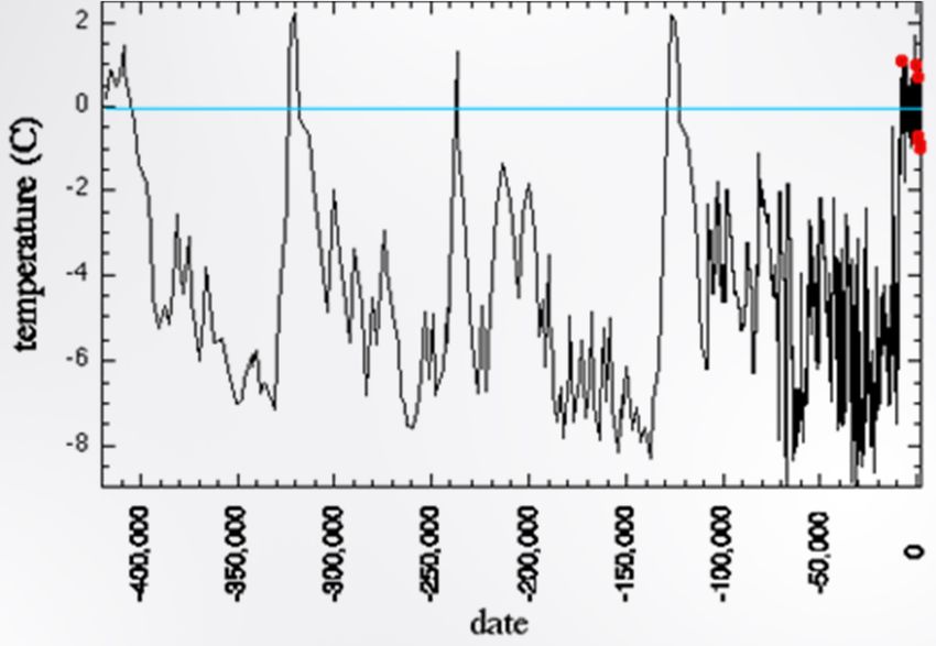
2012 Weather
Winter was very warm except
in Northwest
CDD
HDD
Summer was warm to hot
almost everywhere
High Plains Regional Climate Center (http://www.hprcc.unl.edu)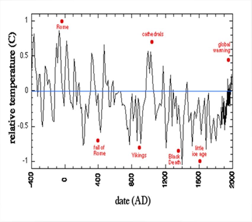
2013 Weather
Winter was cooler than normal in
the North Central
Winter was warmer than normal in
CDD West & Northeast.
HDD
Summer has been cooler than
normal in the Southeast.
Summer has been warmer than
normal in the West
High Plains Regional Climate Center (http://www.hprcc.unl.edu)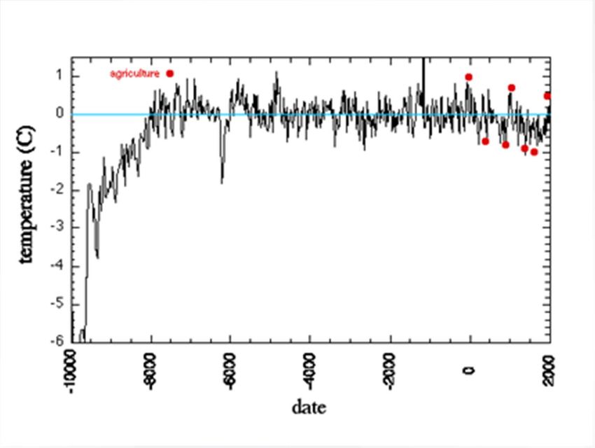
Weather Normalization In a 1% World
» In a slow growth world, it is necessary to have good weather adjustment
  processes to know where the business stands.

                Historical Growth was
                Linear through 2008.
              Annual Gain = 62 TWh/year

                                                     Survey Says:
                                                Annual Gain = 38TWh/year
                                                   About 1% Growth
Why Weather Normalization is Useful
» Actual energy use patterns are erratic. The main source of irregularity is
  weather. This is most obvious at the daily level.

        Actual Daily Energy (MWh)

» Models using normal weather create order out of chaos, providing
  insights about underlying energy use levels and trends.

       Model Predicted Values with Normal Weather
Does your company weather adjust the
following: Monthly sales, Monthly peaks, both
or none?
Applications of Weather Normalization
» Financial forecasting with normal weather
   •   Monthly Budget forecast                            Monthly
   •   Daily budget forecast                              Smooth Daily
   •   Monthly peak forecast                              Monthly peak day & lags
   •   Annual peak forecast                               Annual peak day & lags
» Financial variance analysis
   •   Adjust billed sales                                Cycle month
   •   Adjust billing determinants/revenue by class       Cycle month
   •   Adjust booked sales by class                       Calendar month
   •   Adjust system energy and peak demands              Daily, peak day
   •   Daily tracking of system energy                    Daily
» T&D Facility Planning
   •   8760 hour load forecast for dispatch simulations   Hourly scenario
   •   Design day forecast                                Extreme day
   •   Peak load probability distributions                Multiple scenarios
» Market/Technology Analysis
   •   Typical load profile for a customer                Hourly
   •   Facility baselines for budgets, pricing, ...       Monthly or Daily
Weather Normalization Methods
» All approaches involve use of a model or slope parameters
  developed by modeling historical data.
» There are two general approaches:
    • Normal scenario (define normal weather, then apply model)
         -   Use historical weather to define a set of normal values.
         -   Run normal values through a model to get weather adjusted energy
    • Distributional (simulate multiple weather patterns, then post process)
         -   Run multiple actual weather patterns through a model
         -   Calculate weather adjusted energy from the distribution of model outcomes

» The distributional approach provides a richer set of outcomes allowing
  calculation of means, medians, percentiles and range statistics.
» Claim: If basic principles are followed, the two approaches will provide
  similar results for weather adjustment outcomes.
Why Weather Normalization is Tricky
» The response to weather is nonlinear
• There are low powered degrees
• There are high powered degrees
• The slope is different
» The response varies across seasons
• Slopes are lower in Spring/Fall months
» The response varies across classes
• The point at which cold and warm temperatures start to matter is very different for
small customers than for large customers
» Temperature is the main driver but
• Humidity can matter
• Wind and clouds can matter
• Precipitation can matter
» Weather slopes change over time because of changes in end-
use saturation and efficiency and building efficiencyTypes of Normal Weather
» Daily Normal Degree Days
• Average by date
• Apply nonlinear operations (HDD, CDD) before averaging
» Monthly Normal Degree Days (Calendar and Cycle Months)
• Built up from daily normal (HDD and CDD values)
• Alternatively, compute average of monthly HDD and CDD values
» Peak Producing Weather
• Weather based – hottest, coldest – normal extremes or design day
• Load based – average of weather on historical peak days
» Daily/Hourly Weather Year
• Selected actual weather patterns (TMY -- Typical Meteorological Year)
• Rank and average values daily data by month or season. Assign to calendar
days. Intended to have normal extreme days as well as normal averages
» Simulation Based
• There is no “normal” weather with this approach, just a set of actual weather
years that are simulated through a weather response functionAccounting for Nonlinearities » Temperature is the main driver, and it is very important to recognize the difference between high powered and low powered degrees.
The Model
» The model used in the following examples is a regression model,
  with daily energy as the dependent variable.
» Explanatory variables are:
    •   Calendar month binary variables
    •   Calendar month trend variables                               MAPE = 1.81%

    •   Day of week and specific holiday variables
    •   Multipart weighted CDD and HDD variables for the current day
         -   Estimated weights for low, medium, and high powered degrees
         -   Seasonal weights for spring and fall months
   • Lagged values of multipart weighted CDD and HDD variables.
» The model is estimated with daily data from 2009 to 2012 and is used to
  weather normalize 2012 daily data.
» The results are typical for utilities in the US in 2012
   • Because of the mild spring, winter months are adjusted up
   • Because of the hot summer, summer months are adjusted down
Actual Weather Data is Chaotic
» Actual weather data is chaotic. Some years are less irregular than others.
But all years are irregular. So...what is normal?
Daily Max Temperature
Average of 24 Hourly Values
Daily Min Temperature
Graph shows daily high, low, and average values for one year.Average by Date Method
30 years, daily average temp
For each date, average the 30 values for that date.
Do this for each HDD and CDD variable.Does your company use the Average by Date Method for any of your weather adjustment calculations?
Daily Normal Degree Days -- Average by Date Method
» Compute daily normal HDD and CDD values
• Compute daily average for each day (average of 24 hourly values).
• Compute HDD and CDD values for multiple base temperatures
• Average HDD and CDD values across years for each date
» Smoothing is a good idea for daily tracking calculations
• Compute centered moving average (e.g., 31 day CMA)
• Re normalize to maintain calendar month totals
» This approach is suggested by the simulation approach
• With the simulation approach, a model is evaluated many times for each date (d)
and the simulated loads are averaged
AvgLoadd a b CDD
y 1, 30
y ,d c HDD y ,d 30
• This is algebraically equivalent to the following calculation with DD averages
AvgLoadd a b CDD
y 1, 30
y ,d 30 c HDD
y 1, 30
y ,d 30
• The CDD and HDD averages for a date may both be positive, reflecting that on
that date, there is cooling in some years and heating in others.Degree Day Average by Date
HDD60 -- 30 Year Avg By Date
Individual Year HDD60
CDD60 -- 30 Year Avg By Date
Individual Year HDD60Order of Operation
» When you average by date, the order of operations matters.
» Compute nonlinear transformations (HDD and CDD) first, then average over years.
» Computing HDD and CDD from the averaged values will cause a downward bias in
swing months.
Green line is 30-year
average of HDD55
Values
Green line is 30-year
average of CDD65
Values
Blue line is HDD55
computed from 30 year
average temperature.
Simple example: Red line is CDD65
Two days at 75 and 55 computed from 30 year
Avg Temp = 65 average temperature.
CDD base 65 at Avg Temp = 0
Avg of CDD65 = (10+0)/2
Avg of HDD65 = (0+10)/2What Does Smoothing Do
HDD60 30 Year Avg By Date
Centered MA (31 Days)
Adjusted Centered MA
CDD60 30 Year Avg By Date
Centered MA (31 Days)
Adjusted Centered MASmoothed Daily Normal HDD and CDD » Smoothed and adjusted daily normals look like this. By constructing these values for multiple CDD and HDD cut points, it is possible to distinguish between high powered and low powered degrees in the normalization process.
Average by Date Results
      Actual Daily GWh
      Model using Average By Date
      Model using Avg by Date Smoothed

      Actual Monthly GWh
      Model using Average By Date
      Model using Avg by Date Smoothed
Rank and Average Approach
» Rank and average methods start by creating a “temperature duration” curve.
The first number represents the hottest day in the year/season/month.
» When there are multiple variables, use the main variable (temperature) to
sort the days for all the variables.
Daily High Temperature
Daily Average Temperature
Daily Low Temperature
Graph shows sorted values for one year. Days are sorted by average temperatureRank and Average Process
30 years, daily average temp
Rank and Average by Month
For each year, sort days in each month, hottest to coldest
Average the ranked values in each monthDoes your company use the Rank and Average method for any of your weather adjustment calculations?
2011 and 2012 vs. Rank and Average

               30 years, daily avg temp
               2011 Actual Daily Averages
               30-year Rank and Average

               2012 Actual Daily Averages
               30-year Rank and Average
2013 Through August vs. Rank and Average
2013 Actual Daily Averages
30-year Rank and AverageOrdering the Rank and Average Data
» Rank and average data represent typical extremes as well as typical
averages.
» Once the rank and average values are calculated, they must be assigned to
a calendar.
• Where does the hottest day go in each month
• Where does the coldest day go in each month
• Where do the seasonal peak days go in each season
• How do we rotate this to multiple years
» Approaches to ordering include
• Select a “typical” year and use that order
• Get typical meteorological year (TMY) data and use that order
• Use the order that occurred in the year being normalized
» There is no “correct” way to assign the data to a calendar
• The result will always be an erratic pattern
• An erratic pattern is required to represent the extremes and to generate a
realistic hourly profileOrdering by 2012 Pattern
Rank and Average By Season
Rank and Average By Month
Average by Date
Actual 2012 Daily Average
Rank & Average Ordered by 2012 PatternRank and Average Energy Results
Actual Daily GWh
Model using Avg By Date Smoothed
Model Rank & Avg Ordered by 2012
Actual Monthly GWh
Model using Avg by Date Smoothed
Model Rank & Avg Ordered by 2012Simulation Approach
» Use each historical year of weather to simulate loads and weather
adjustments.
» Possibly shift weather forward and backward by 1, 2, 3, … days
» Each pattern and shift generates a full set of hourly, daily, monthly results
» This is a good way to understand weather uncertainty
» This is the best way to understand the impact of weather diversity in large
geographies
30 years, daily average tempDoes your company use the Simulation Method for any of your weather adjustment calculations?
What You Get from the Simulation Approach

   Simulated loads for 30 weather years
   Avg of 30 Simulated Loads

   2012 Weather Adjustments for 30 years of weather
   Avg of 30 Weather Adjustments
Comparison of Results from Simulation Approach

    Model using Average by Date
    Avg of 30 Simulated Loads

    Actual Monthly GWh
    Model using Avg by Date
    Avg of 30 Simulated Loads
Simulation Method Results
» The simulation approach also provides a distribution of results that would
have occurred with different actual weather patterns.
» The is very useful for understanding the range of possible outcomes based
on alternative weather patterns.
» This can be used to parameterize uncertainty related to weather. Uncertainty
can also be parameterized using weather slopes and measures of HDD and
CDD uncertainty.
Mean
Median
2012
Actual
Cumulative Probability
For Annual Sales
2012 Monthly Energy with 30 Years of Weather
Average of 30 Weather Simulations
2012 Monthly Energy
Annual Sales (TWh)Simulation Distributions for Peaks » Example from 1978
Validation Using Neural Network Simulations
» As a final comparison, a neural network model is used to implement
  the simulation approach.
» Neural networks provide a flexible nonlinear modeling framework
  that do not rely on any assumptions about linearity or degree day
  bases.
» The specification includes the following
   • Linear node with monthly binary variables, monthly trend
      variables, day of week binary variables, and holiday binary
      variables.
   • Nonlinear nodes with current day average temperature, lag day
      temperatures, and monthly binary variables.
» The model is estimated with data from 2009 to 2012 and simulated
  with actual historical weather patterns from 2003 to 2012.
Comparison of Results from Neural Network Simulations
Actual Monthly GWh
Avg of 30 Simulated Regressions
Avg of 30 Simulated Neural Nets
Actual Monthly GWh
Avg of 30 Simulated Regressions
Avg of 30 Simulated Neural NetsConclusions on Method
» Models that recognize that load response is nonlinear are required
» Multi-part linear (spline) models are good for this
• For system load
• For rate classes using weights from load research models
» The three main methods are
• Average by date
• Rank and average
• Simulation
» They will give similar results if the modeling and data processing are done
correctly (annual adjusted energy within .02% in the example)
• Average by date is good for cycle and calendar month
energy normalization and daily tracking against a smooth
normal
• Rank and average is good for calendar month energy
normalization and for generating an 8760 for production cost
simulations
• Simulation approach is good for energy normalization and
for generating uncertainty bands (e.g., 90/10 outcomes).How many years of historical weather data do you use to define normal weather?
Current Practice – Number of Years

  » Between 2006 and 2013 there is a general shift to use fewer years
    when calculating normal weather
      • 2006 Survey included 172 Respondents
      • 2013 Survey included 53 Respondents
The Last 2,400 Years
1880 on from NOAA area weighted average of earth temperatures.
Pre 1880 from Greenland Ice Sheet Project (GISP2) calibrated to post 1980 data.The Last 10,000 Years
1880 on from NOAA area weighted average of earth temperatures.
Pre 1880 from Greenland Ice Sheet Project (GISP2) calibrated to post 1980 data.The Last 400,000 Years
1880 on from NOAA area weighted average of earth temperatures.
Pre 1880 from Greenland Ice Sheet Project (GISP2) calibrated to post 1980 data.2013 Brown Bag Seminars » Solar and Wind Generation Modeling and Forecasting - March 5 » 2013 Forecast Accuracy Benchmarking Survey and Energy Trends - June 4 » Update on Weather Normalization Trends and Issues - Sept 17 » 2014 Outlook - Dec 10, 2013 All at noon, Pacific Time All are recorded. PDF and recording available after the session.
Press *6
Questions?                                         to ask a question
Remaining 2013 HANDS-ON WORKSHOPS
» Forecasting 101
  – October 22-24 - San Diego, CA
» Fundamentals of Sales and Demand Forecasting
  – October 29-30 - Boston, MA

OTHER FORECASTING MEETINGS
» Itron Utility Week – October 7-8 – Orlando, FL

    For more information and registration:
    www.itron.com/forecastingworkshops
    Contact us at: 1.800.755.9585, 1.858.724.2620 or
    forecasting@itron.com
You can also read