Working Paper Series LSIs' exposures to climate change related risks: an approach to assess physical risks - European ...
←
→
Page content transcription
If your browser does not render page correctly, please read the page content below

Working Paper Series
                           Maria Sole Pagliari   LSIs’ exposures to climate change
                                                 related risks:
                                                 an approach to assess physical risks

                                                   No 2517 / January 2021

Disclaimer: This paper should not be reported as representing the views of the European Central Bank
(ECB). The views expressed are those of the authors and do not necessarily reflect those of the ECB.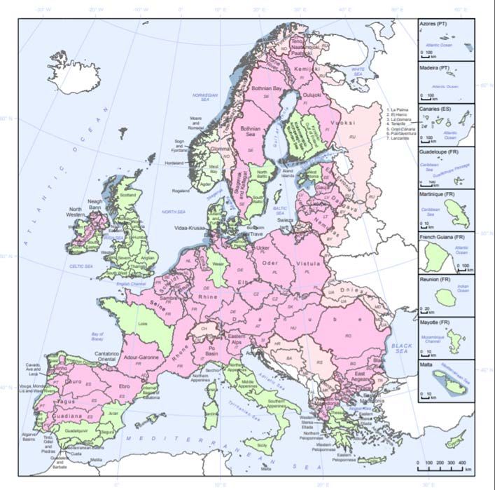
Abstract
       This paper proposes an approach to estimate the impact of adverse climatic events on the
       profitability of small European banks (LSIs). By considering river flooding phenomena, we
       construct a unique database matching the information on location, frequency and severity of
       floods with the location and balance sheet data of institutions mainly operating in the areas
       where they are headquartered (territorial LSIs). We compare the performance of territorial
       LSIs across regions at low and high flooding risk and test for the “core lending channel”
       hypothesis, whereby lending to the real economy is a catalyst of physical risks. Results show
       that an adverse event dropping loans to households and non-financial corporations by one
       percentage point (pp) of total assets entails a decrease in the Return on Assets (ROA) of
       territorial LSIs in riskier areas by 0.01pps (~3.1%). Moreover, if all territorial LSIs were
       located in riskier areas, one bank out of two would report an average ROA between 0.0001
       and 0.52 percentage points lower than what observed.

       JEL codes: C33, G21, Q54
       Keywords: Climate change, LSIs, Profitability, Dynamic panel regressions, Core Lending

ECB Working Paper Series No 2517 / January 2021                                                        1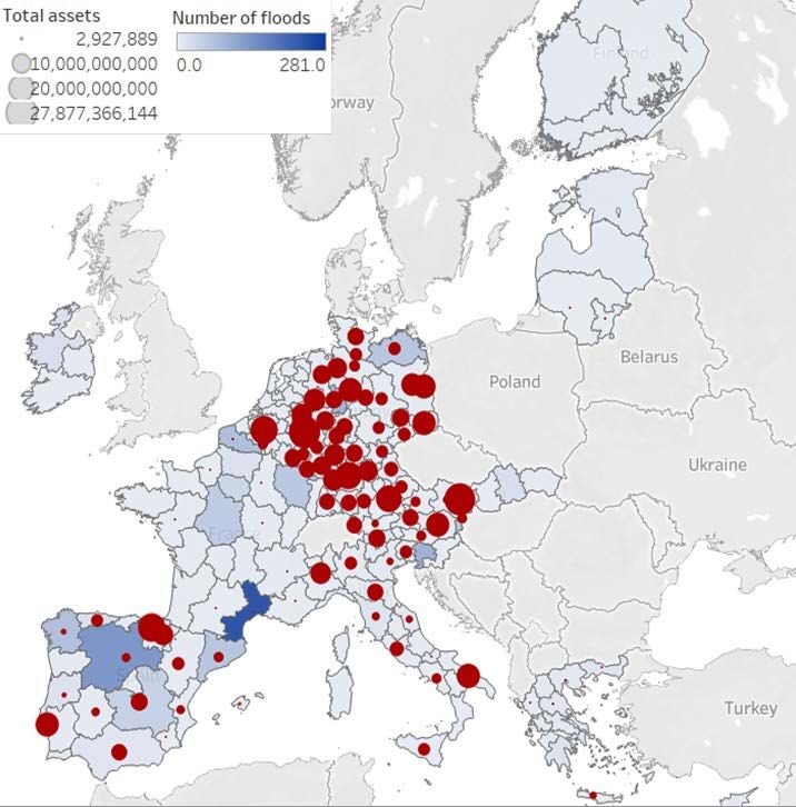
Non-technical summary

The topic of how climate change might affect the performance of the financial sector has gained
increasing attention in the private sector as well as in policy fora, and is urging an adequate
response. This paper relates to the current debate by assessing the possible effects of climate-
change related risks on the performance of European Less Significant Institutions (LSIs).
An evaluation of these risks is made difficult by the lack of information about the geographical
location of customers’ businesses, their collaterals and the coverage provided by insurance poli-
cies. We propose an approach that leverages on the specificity of some LSIs business models.
Institutions like credit cooperative and savings banks, for instance, are by nature more linked
to the territory where they are headquartered. A large share of the exposures of these LSIs
towards the real economy is therefore vis-à–vis counterparts that are geographically close to the
bank. Data on their lending book should then be a good approximation of the geographical
concentration of exposures.
This paper takes into consideration one of the most prominent sources of physical risks, namely
floods (coastal, fluvial and pluvial), since these types of adverse events are expected to rise as a
result of climate change. In particular, river floods are common natural disasters in Europe and
are among the most important hazards in terms of economic damage. Notably, information on
location and severity of flooding phenomena over time are associated to the location informa-
tion at our disposal for European LSIs. These elements are then associated to additional data
regarding the banks’ business model, as well as key balance sheet metrics from ITS reporting.
The dataset thus constructed is unique in its structure and would allow to approximate, to a
reasonable extent, the potential exposure of territorial LSIs to flood risks, working under the
assumption that these banks are by definition more anchored to their territory compared to
others.
We then use the database to quantify the potential effects that an increase in flood risks might
have on the performance of territorial LSIs. In particular, we focus on the role played by loans
to the real economy as a catalyst for the materialisation of these risks on banks’ balance sheets.
Results show that a decrease in loans to households and non-financial corporations over total
assets by one percentage point leads to an average drop in a territorial bank’s Return on Assets
(ROA) by 0.007 percentage points (1.9% of the average ROA), this negative effect being even
bigger for LSIs in areas subjected to more severe floods (0.011 percentage points, or 3.1% of
the average ROA). Via a counterfactual experiment, we finally show that if all territorial LSIs
were located in risky areas, one out of two banks in the sample would have a lower profitability,
with average decreases in ROA ranging between 0.0001 and 0.52 percentage points.

ECB Working Paper Series No 2517 / January 2021                                                   2
1       Introduction

The topic of how climate change might affect the performance of the financial sector has gained
increasing attention both in the private sector as well as in policy fora, and is urging an adequate
response1 .
This paper relates to the current debate by assessing the possible effects of climate-change
related risks on the performance of European Less Significant Institutions (LSIs). In particular,
a special category of such risks, physical risks, refer to direct losses caused by climate events
and can be classified as:

     i) chronic risks (e.g., rising sea levels and increasing temperatures);
    ii) occurrence of extreme weather events (e.g., heavy rainfalls and hurricanes).

Between these two types, the negative impact of extreme events is relatively easier to assess, in
that the effects of chronic risks are much more gradual over time. We then focus on this specific
typology of climate-related risks.
Physical risks can impact the banking sector via an increase in:

     i) credit risk, stemming from the banks’ exposures to households, companies and financial
        counterparts that can default on their obligations;
    ii) market risk, deriving from sudden adverse movements in market prices;
    iii) operational risk, resulting from inadequate or failing internal processes, people and systems
        or from external events.

Among them, credit risk is particularly relevant for those LSIs with more traditional business
models (e.g., retail banks) and it can materialise via:

     i) a worsening of the borrowers’ repayment capacity;
    ii) a direct damage to physical collaterals.

Therefore, the present analysis takes into consideration how a well-defined category of physical
risks, i.e. flooding events, can affect the profitability of smaller European banks via a change
in credit risk, thus fitting into a wide stream of ongoing research (Giuzio et al. (2019), Carbone
et al. (2019), Schellekens and van Toor (2019), Vermeulen et al. (2018))2 .
It is commonly accepted that the materiality of physical risks is still low due to wide insur-
ance coverage as a first line of loss absorption (ACPR (2019a,b,c)). Banks would be hit only
    1
     See in this regard the European Commission’s Action plan on Financing Sustainable Growth, released in
March 2018 and the EBA’s Action Plan on Sustainable Finance released in December 2019.
   2
     In a similar vein, Sautner et al. (2020) propose an alternative approach to measure firm-level climate change
exposure from conversations in the earnings conference calls.

ECB Working Paper Series No 2517 / January 2021                                                                 3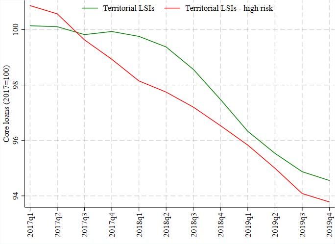
indirectly and for the residual losses not covered by insurance policies. Nonetheless, such a
statement crucially depends on the geographical composition of the banks’ assets portfolios.
There are indeed areas in Europe that are more exposed to climate-related physical risks and
this might generate substantial issues for institutions with higher credit exposures in those ar-
eas. However, an assessment of these risks is made difficult by the lack of information about
the geographical location of customers’ businesses, their collaterals and the degree of coverage
of insurance policies.
The approach proposed in this paper leverages on the specificity of some of the LSIs business
models. Institutions like credit cooperative and savings banks, indeed, are by nature more
linked to the territory where they are headquartered3 . A large share of the exposures of these
LSIs (territorial LSIs henceforth) towards the real economy (e.g. non-financial corporations
and households) is therefore vis-à–vis counterparts that are geographically close to the bank.
Territorial LSIs can hence represent an ideal grouping to produce a first quantitative assessment
of the effects of climate-related risks.
Against this backdrop, data on their lending book should provide, to a good degree of ap-
proximation, an indication of the geographical concentration of exposures. Given this working
hypothesis, the first part of the paper will focus on providing some stylized facts about the
credit that these banks have towards households (HHs) and non-financial corporations (NFCs),
as adverse climatic events might take a higher toll onto the repayment capacity of these coun-
terparts, thus making them more vulnerable to physical risks. In this regard, the literature
has also highlighted the negative relationship between climate-related transition risks and the
creditworthiness of loans and bonds issued by corporates (Delis et al. (2019), Capasso et al.
(2020)).
One of the most prominent sources of physical risks is given by floods (coastal, fluvial and
pluvial), in that these adverse events are expected to rise as a result of climate change (BOE
(2018)). In particular, river floods are a common natural disaster in Europe and are among
the most important hazards in terms of economic damage. River floods can indeed provoke
substantial losses deriving from direct and indirect damages to infrastructure, property, agri-
cultural land and production4 . Moreover, part of the existing literature has highlighted the
existence of a negative relationship between flood risk exposure and lending to NFCs and HHs
(Faiella and Natoli (2018), Garbarino and Guin (2020)). The first step of the analysis will then
   3
      In this regard, the European Economic and Social Committee (EESC) has stated that: “[. . . ] cooperative
and savings banks offer some highly distinctive features: these include their links with the local production
fabric, their firm anchorage in their region, [. . . ], their closeness to local interests and social operators, and their
solidarity” (EESC (2015)).
    4
      See https://www.eea.europa.eu/data-and-maps/indicators/river-floods-3/assessment.

ECB Working Paper Series No 2517 / January 2021                                                                         4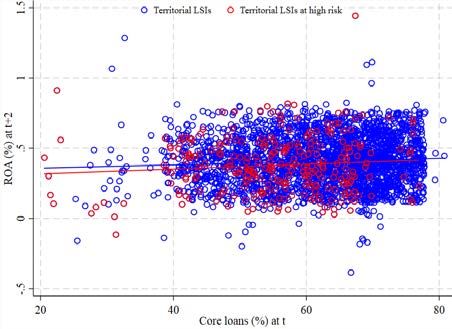
consist of evaluating the concentration of territorial LSIs in regions that are more exposed to
severe flooding phenomena.
All the results discussed in the following sections build on the information collected about the
frequency and severity of flood events in the 19 SSM countries over the period 1980-2014, as
provided by the European Environment Agency (EEA)5 . Notably, the dataset matches data on
the location of the events, as well as their intensity and duration, with the locational information
at our disposal for European LSIs. These elements are associated to additional data regarding
the banks’ business model and to the key balance sheet metrics from ITS reporting over the
period 2018Q1-2019Q46 . The dataset thus constructed is unique in its structure, in that it ap-
proximates, to a reasonable extent, the potential exposure of territorial LSIs to flood risks, given
the assumption that these banks are by definition more anchored to their territory compared
to others. An additional caveat to our analysis consists of approximating the exposure to flood
risks by looking at the historical occurrence of flooding phenomena, a choice motivated by the
empirical regularities characterizing the observation of these events, as explained in Section 27 .
The paper is structured along two main blocks. In the first part, we define the concept of
territorial LSIs and we identify those banks for which flooding risks might be more relevant.
Besides the more immediate supervisory use8 , the first part is instrumental for conducting a
more structural analysis aimed at exploring how physical risks can materialise on banks’ bal-
ance sheets. Notably, in Section 3 we first provide an overview of the possible mechanisms of
transmissions and, then, set up a panel regression model to analyse the relationship between
flood risks, lending to the real economy and LSIs profitability. We find that the “core lending
channel” is more relevant for territorial LSIs than for other types of institutions and this is es-
pecially the case when taking into consideration those banks located in areas at higher flooding
risk. A decrease in loans to households and non-financial corporations by one percentage point
with respect to total assets leads to an average drop in a territorial bank’s return on assets
(ROA) by 0.007 percentage points (1.9% of the average ROA), this negative effect being even
more pronounced at LSIs in areas subjected to more severe floods (0.011 percentage points, or
3.1% of the average ROA at these institutions).
We finally perform a counterfactual exercise to show that, if all territorial LSIs were located in
risky areas, their profitability would be significantly lower with a probability of 50% (one out
   5
     The database is being currently updated with information until 2019.                          Refer also to
https://www.eea.europa.eu/data-and-maps for a list of publicly available datasets.
   6
     The period of reference is reduced to the time span where LSIs report the complete FINREP and CoRep
templates.
   7
     In this regard, a report by the UK Committee on Climate Change (CCC) highlights that extreme floods like
the ones experienced in UK in Autumn 2000 are to become more and more frequent in future (CCC (2016)).
   8
     This list of banks can be submitted to line supervisors, who can then follow up with their respective banks
and check whether an institution has adopted special strategies to internalize flood risks in its portfolio.

ECB Working Paper Series No 2517 / January 2021                                                               5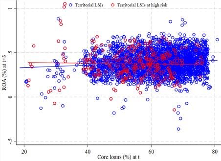
of two banks in the sample), with average decreases in ROA ranging between 0.0001 and 0.52
percentage points. In particular, we identify 350 banks whose ROA would drop on average by
0.17 percentage points, from 0.45% to 0.28%, and that account for around 29% of total LSI
sector’s assets.

2       Relating floods and banks data

This section provides an overview of the selection algorithm deployed to identify the sample of
European territorial LSIs that are more vulnerable to severe river floods. In particular, Sec-
tion 2.1 analyses the flood database and describes the key features of the events. Section 2.2 then
relates this information to the bank-level dataset to identify the group of banks in potentially
riskier areas.

2.1     Identification of areas at higher flood risk in Europe

The first step consists of analyzing the main trends emerging from flood data, both in terms of
frequency and severity, with the purpose of identifying geographical areas more subject to this
risk. Figure 1a depicts the evolution of the euro area aggregate number of reported floods over
time. At a first glance, the time series shows a certain degree of fluctuation in the occurrence
of events, though featuring a clear upward trend which is generally more evident for the more
severe episodes (Figure 1b)9 .

Figure 1: Flood events in the euro area.
          (a) Number of flood events by year                 (b) Time trends for flood events by intensity

Source: EEA, author’s computations.
Notes: Time trends are estimated over the period 1980-2010. Shaded areas represent 95% confidence bands.

Aggregate data however conceal a great degree of cross-country heterogeneity, both in terms of
    9
    Fluctuation in the number of events is also due to the different country coverage, which raises significantly
after the year 2000, when first data from CEE countries became available. The database is also less complete
after the year 2010, when the number of reported events falls sharply.

ECB Working Paper Series No 2517 / January 2021                                                                6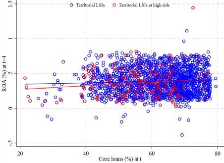
total number of reported events and as regards the severity of such events. For instance, large
countries like France, Germany and Spain account for more than 70% of the total number of
reported events (Figure 2a)10 . Meanwhile, in countries like Finland, Latvia and the Netherlands,
although the total number of events is lower, such events are particularly severe (Figure 2b).
This is also the case of Italy, which is the country among the largest ones to report the lowest
number of events.
Figure 2: Flood events by country.
               (a) Number of flood events                              (b) Intensity of flood events

Source: EEA, author’s computations.

The following analysis will then take into account these differences when evaluating LSIs’ activ-
ities in the different territories. In this regard, flood data are collected along the geographical
classification by River Basin Districts (RBDs), rather than along the administrative boundaries.
This often entails that single RBDs correspond to multiple NUTS regions. When that is the
case, it is assumed that each NUTS region embedded in one RBD has been subjected to the
same number of events as reported in the whole RBD.
In order to better identify the potential effects that flood risks can exert onto LSIs’ credit
exposure, the analysis focuses only on those areas of Europe that are particularly exposed to
floods. In particular, in each country higher flood risk regions are identified as those where
the number of severe events (corresponding to intensity “high” or “very high”) is one standard
deviation higher than the average of the country where these regions are located. This relative
classification takes into account the cross-country heterogeneity in terms of reporting policies
and enable to identify risk areas in each of the 19 SSM jurisdictions. The proposed approach
identifies a total of 19 regions subjected to high risk and 18 exposed to very high risk, over a
total of 173 regions across Europe. By the same approach, we detect 17 regions that have been
subjected over time to relatively more frequent high or very high-intensity floods. A check of
  10
     This is also partly due to a reporting bias, as some national agencies are more inclined to report lots of low
severity events. Descriptive statistics computed only for countries that have more rigorous reporting over time
(e.g., France, Germany, Italy and Spain), however, show the same trends detected with aggregate figures.

ECB Working Paper Series No 2517 / January 2021                                                                  7
the higher-moments of the empirical distribution of flood events (Table 1), as well as a visual
inspection of the kernel densities (Figure 4) show that our approach well captures the higher
tail of the risk distribution.
Table 1: Descriptive statistics of flood events by intensity
                                            High                                                    Very high                                      High and very high
 Country          (1)       (2)         (3)      (4)        (5)     (6)      (1)         (2)         (3)     (4)         (5)   (6)     (1)     (2)     (3)      (4)       (5)   (6)
 AT              2.00      4.56         2.36     6.80      6.56      1      4.11        8.99        2.44    7.02       13.10    1     6.11   13.52     2.43    7.00     19.63    1
 BE              0.27      0.47        1.02      2.04      0.74      3      1.64        2.11        1.57    4.79        3.75    1     1.91    2.30     1.77    5.58      4.21    1
 CY              2.00        -            -        -       2.00      0      0.00          -           -       -         0.00    0     2.00      -        -       -       2.00    0
 DE              0.61      1.50         3.09    12.01      2.10      3       3.89       9.16        3.81   17.60       13.06    3     4.50   10.47     3.63   15.83     14.97    3
 EE             6.00         -            -        -       6.00      0       1.00         -           -       -         1.00    0     7.00      -        -       -       7.00    0
 ES             14.58     30.74        2.36      7.07     45.32      2      14.05      19.17        1.21   2.93        33.22    5    28.63   47.78     1.95   5.66      76.41    2
 FI             0.25      0.50          1.15     2.33      0.75      1       1.25       0.96       -0.49    1.63        2.21    0     1.50    1.29     0.00    1.64      2.79    1
 FR              3.43      8.43        3.26     13.55     11.87      2       4.91      12.89        3.84   17.07       17.81    2     8.35   21.11     3.69   16.21     29.46    1
 GR              0.92      1.26         1.20     3.59      2.18      1       2.38       2.63        0.99    3.03        5.02    2     3.31    3.54     0.69    2.20      6.85    3
 IE              2.00      3.46         0.71     1.50      5.46      1       3.00       1.00        0.00    1.50        4.00    0     5.00    4.36     0.67    1.50      9.36    1
 IT              0.14      0.36         2.04     5.17      0.50      3       2.86       2.74        2.10    7.27        5.60    2     3.00    2.86     2.34    8.40      5.86    2
 LT             0.00         -            -        -       0.00      0       0.00         -           -       -         0.00    0     0.00      -        -       -       0.00    0
 LU              0.00        -            -        -       0.00      0       0.00         -           -       -         0.00    0     0.00      -        -       -       0.00    0
 LV              1.00        -            -        -       1.00      0       2.00         -           -       -         2.00    0     3.00      -        -       -       3.00    0
 MT              0.00        -            -        -       0.00      0       0.00         -           -       -         0.00    0     0.00      -        -       -       0.00    0
 NL              0.75      0.45        -1.15     2.33      1.20      0       1.00         -           -       -         1.00    0     1.75    0.45    -1.15    2.33      2.20    0
 PT             0.14      0.38          2.04     5.17      0.52      1       2.43       3.87        1.85    4.76        6.30    1     2.57    3.82     1.80    4.68      6.39    1
 SI             19.00     26.87         0.00     1.00     45.87      0       8.50       9.19        0.00    1.00       17.69    0    27.50   36.06     0.00   1.00      63.56    0
 SK              2.00      2.71        1.05      2.26      4.71      1       3.50       4.51        0.91    2.12        8.01    1     5.50    7.14     1.03    2.22     12.64    1
 Total           2.82     11.67        7.06     57.35     14.48     19      4.34        9.91        3.95   19.08       14.25   18     7.16   20.18     5.38   36.10     27.33   17
         (1)            (2)                             (3)               (4)               (5)                (6)
Notes:         Mean;          Standard deviation;             Skewness;         Kurtosis;         Threshold;         Number of identified regions with extreme frequency.

Figure 3: Kernel density of reported events and frequency by intensity.
                                      70

                                                                                                                                                   70
                                      60

                                                                                                                                                   60
                                      50

                                                                                                                                                                 50
                                                                                                                                                   Frequency (%)
                                 Density (%)
                                         40

                                                                                                                                                           40
                                  30

                                                                                                                                                     30
                                      20

                                                                                                                                                   20
                                      10

                                                                                                                                                   10
                                      0

                                                                                                                                                   0

                                               0                     5                            10                      15                  20

                                                                    Total (lhs)                        High
                                                                    Very high                          Combined high + very high

Source: Author’s computations.

2.2        Identification of LSIs exposed to flood risk

The sample of European LSIs that is considered for the purpose of the paper is given by those
institutions with a typically stronger territorial focus, i.e., those banks that are likely to operate

ECB Working Paper Series No 2517 / January 2021                                                                                                                                   8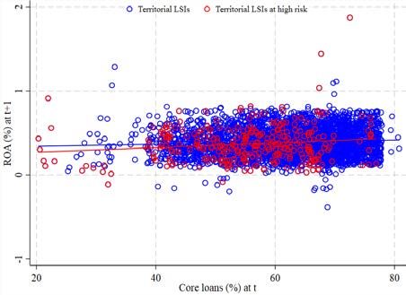
in the territory where they are headquartered. This territorial focus might make institutions
more vulnerable to sudden adverse flooding events in geographical areas that are more prone
to these events. An example of such type of banks (territorial LSIs henceforth) is given by
those LSIs operating within the credit cooperative and savings sectors11 . All in all, 1718 LSIs
are considered over 9 SSM countries, which make more than a half of the entire LSI sector
in terms of total assets (64%)12 . Among these banks, around 131 operate in areas that are
particularly exposed to severe floods, as revealed by the historical records of events in those
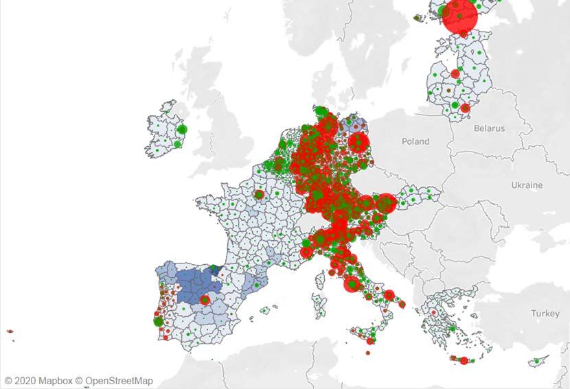
regions, while 126 LSIs are located in areas exposed to milder flooding risks. Figure 4 depicts
the concentration of more severe flood episodes across the euro area, together with the location
of territorial LSIs.
Figure 4: Intensity of floods by NUTS region and “territorial” LSIs.
Source: EEA, ECB supervisory statistics, author’s computations.
Notes: Bubbles dimension is proportional to the assets size of the related LSI.
11
See Appendix B for more details about the selection of territorial LSIs
12
These numbers are based on a sample of banks fixed at 2019Q4. Using a changing composition approach
would enlarge the sample to 1738 institutions. The results reported in the following analyses, however, do not
substantially change across the two sampling methodologies.
ECB Working Paper Series No 2517 / January 2021 9One of the major channels whereby these risks can affect LSIs performance is given by their
credit exposure towards the real economy, especially lending to both non-financial corporations
(NFCs) and households (HHs). These particular counterparts are indeed more vulnerable to a
rise in the frequency and severity of floods in the regions where they operate/reside. Absent
more comprehensive information on the location of counterparts, an indication of the potential
exposure of territorial LSIs to risks related to flooding is provided by the amount of loans they
have booked on their balance sheets towards NFCs and HHs, assuming that the geographical
scope of business for these banks is circumscribed by the region where they are located13 .
Figure 5 shows aggregate figures for loan stocks to HHs and NFCs in 2019Q4 by LSIs located
in regions with moderate, high and very high flooding risk. All in all, territorial LSIs operating
in higher flood risk regions at the end of 2019Q4 held an amount of loans to the real sector
corresponding to 4.56% of total LSIs loans to HHs and NFCs, which drops to 4.21% when
considering also loans to other banks, non-bank financial corporations and the government
(Table 2).
Figure 5: Share of territorial LSIs loans by flood Table 2: Territorial LSIs in risky areas by coun-
intensity try
Country # Total Loans “Core” Loans
DE 54 4.07% 4.21%
IT 43 9.45% 10.92%
AT 23 2.60% 2.08%
ES 5 19.78% 24.09%
PT 4 1.97% 1.18%
BE 1 4.83% 5.82%
FR 1 0.07% 0.07%
Total 131 4.21% 4.56%
Source: ECB supervisory statistics, author’s com-
Source: ECB supervisory statistics, author’s computa- putations.
tions. Notes: Data refer to 2019Q4. # refers to the
Notes: Data refer to 2019Q4. Bars represent percent- number of banks headquartered in the identified
age shares of total loans, while the solid line reports total riskier areas. Total loans include loans to HHs,
loans in EUR bn (rhs). NFCs, other financial corporations, banks and the
government. “Core” loans refer to the amount of
loans to HHs and NFCs as a share of the total.
Out of these 131 institutions, 54 are located in Germany and account for around 5% of the
domestic LSI sector’s loans to the real economy. The second most represented country is Italy,
with 43 banks accounting for almost 15% of the domestic LSIs’ loans, while the third is Austria
(23 for a total 4% of domestic loans). Out of the remaining 11 banks, 5 are located in Spain
13
Other types of assets could also be exposed to such risks, like for instance equity or traded debt of companies
with large share of their operations located in or near areas subject to flood risks. However, the amounts of these
assets on territorial LSIs’ balance sheets are typically much inferior to loans.
ECB Working Paper Series No 2517 / January 2021 10and account for 10% of domestic “core” loans, 4 are in Portugal (4.2%), 2 (one each) in Belgium
(18%) and France (0.14%).
3 Banks’ profitability, flood exposure and the lending channel
In this section we provide some evidence on the impact of flood risks onto LSIs profitability. As
mentioned in Section 1, one of the main channels of transmission of physical risks to the banking
sector is given by an increase in credit risks. Such risks can have a repercussion on banks’
profitability via changes in elements of the income statement. For instance, a deterioration in
the borrowers’ repayment capacity can entail a decrease in the net interest income deriving from
a reduction in performing loans, or an increase in provisioning in anticipation of higher default
probabilities. Both these instances can lead to a decrease in profits and, hence, profitability.
Against this backdrop, banks headquartered in areas that are more subjected to floods might
also internalize physical risks by adopting some mitigation measures aimed at increasing their
loss absorption capacity (e.g., via an adjustment of their pricing schedule so to charge higher
interests on loans to HHs and NFCs in those areas or via an increase in liquidity and capital
buffers)14 .
Our analysis mainly focuses on the dynamics that flood risks can trigger in the profit and losses
statement of territorial LSIs. The working hypothesis which our analysis rests upon is that a
higher amount of exposures to HHs and NFCs at a given point in time is likely to make banks
located in risky areas more vulnerable to the economic damage deriving from a severe flood.
This assumption is directly derived from the peculiar characteristics of the banks we focus on,
i.e. small institutions whose business is concentrated in areas surrounding their headquarters. In
other words, the setup adopted in the following sections is devised to quantify the repercussions
of flood risks on a well-defined category of banks, territorial LSIs, via a particular transmission
channel, i.e. credit risk on the banks’ balance sheet.
A more direct approach (e.g., regressing ROA on the number of past severe flooding events)
would make it not possible to disentangle across different transmission channels. In addition,
the historical information on river floods, while being indicative for the risk in each territory,
predate the available ITS data for LSIs, which de facto does not allow for a straight temporal
comparison between flood events and banks’ performance. Nonetheless, one of the robustness
checks in Appendix C.2 proposes a regression setup similar to Murfin and Spiegel (2020). Not
only are the results aligned with those of the baseline regression, but we also find that including
the historical number of floods among the control variables makes the coefficient on core loans
14
On the effects of physical risks on pricing, see also Bernstein et al. (2019).
ECB Working Paper Series No 2517 / January 2021 11significantly higher, which further supports our assumption that flood risks take a toll onto LSIs performance mainly through core lending. 3.1 Preliminary evidence Figure 6 depicts the distribution of the average ROA across the LSI banks in the sample. While the pooled empirical distribution of ROA (Figure 6a) at LSIs potentially more exposed to severe flooding is not significantly different compared to the other LSIs, on the other hand an analysis of the distribution over time (Figure 6b) reveals that the same institutions have reported on average a lower ROA compared to the other LSIs, though the gap between the two groupings has closed since 2019Q3. This is also reflected by the lower mean of ROA at LSIs in riskier areas (0.34%) compared to other territorial LSIs (0.37%), a difference (6%) which is statistically significant at the 1% significance level. A cross-country comparison of ROA distribution reveals that such discrepancy is mainly driven by countries like Austria, Portugal and, to a lesser extent, Germany, while the contrary holds true in Italy and Spain (Figure 6c). So far, empirical evidence hints at a difference in performance among territorial LSIs identified as more or less exposed to flood risks, though this cannot be interpreted as a straight causal link between flood risk exposure and profitability. Notably, it is necessary to adopt a structural approach to gauge a more precise indication of the underlying mechanisms at play. Table 3 provides a comparison of some bank-level aggregates across territorial LSIs. The lower average ROA in areas at higher risk is generally associated with inferior lending to HHs and NFCs, lower net interest margins, higher provisions, core interest income, cost-to-income ratio and TIER1 capital ratio. These stylized facts seem to suggest that flood risks can impact profitability in two ways: i) via an increase in credit risk, as reflected by the drop in net interest margin and the increase in provisioning; ii) via the deployment of mitigation measures (e.g., more expensive pricing and greater capital buffers). As regards the link with the amount of loans to HHs and NFCs that territorial LSIs hold on their balance sheets, a quick glance at the available data suggest that core lending has generally decreased at these institutions, in particular in 2018. However, it also looks like that the decline has been slightly more marked at LSIs located in areas at higher flood risk (see Figure 7). Moreover, Figure 8 displays the results of simple regressions of banks’ ROA on the amount of loans to HHs and NFCs in the preceding quarter, at different horizons. Although this exercise does not control for the mechanisms discussed above, estimates already provide useful insights. For horizons from 1 to 4 quarters ahead, indeed, the relationship between ROA and the amount of core loans is positive and marginally more marked at those territorial LSIs belonging to the ECB Working Paper Series No 2517 / January 2021 12
Figure 6: Profitability at LSIs
             (a) Pooled distribution of ROA                            (b) Distribution of ROA over time

                                        (c) Distribution of ROA by country

Notes: charts are based on a fixed sample of LSIs that have constantly reported their balance sheet positions
over the period 2018Q1-2019Q4. This explains why there are no statistics for the French riskier LSI in Figure 6c.
In Figure 6b, solid lines represent medians, while shaded areas mark 16%-84% (dark gray) and 10%-90% (light
gray) percentiles.
Source: ECB supervisory statistics, author’s computations.

riskier batch. This seems to suggest that: i) profitability at territorial LSIs is more sensitive
to changes in core lending; ii) the link is stronger for territorial LSIs in areas at higher risk of
floods. This in turn would suggest that a sudden drop in the performance status of such loans
due to a severe flooding would have a more pronounced impact on the ROA.
This statement, however, abstracts from any consideration regarding the possible side-effects
stemming from an increase in provisions or a decrease in the net interest income, as well as
the impact of the mitigation measures15 . We therefore explore this “core lending channel” in
  15
     Provisioning is one of the first lines of defense for banks to internalize shifts in risks, especially credit risks.
For this reason, part of the banking literature takes provisions as the main variable of interest. However, such
approach is not particularly suitable for the LSIs we focus on, in that most of them belong to jurisdictions (e.g.,
Germany and Austria) where the accounting framework allows to substitute provisions on the income statement
with capital buffers (hidden reserves) that are not directly reported on the balance sheet. This in turn entails
an artificially low level of provisions that is not commensurate to the real on-balance-sheet risks, thus making it
difficult to perform a meaningful analysis of the link between lending and provisioning.

ECB Working Paper Series No 2517 / January 2021                                                                       13
Table 3: Averages of bank-level variables at territorial LSIs
Variable Territorial LSIs Territorial LSIs
at low risk at high risk
ROA (%) 0.37 0.34
Total assets (log) 20.19 20.01
Core loans (%) 62.21 55.10
Net Interest Margin1(%) 1.04 0.99
Provisions (%) 0.00 0.01
Core interest income2(%) 92.97 96.22
Cost-to-income ratio3(%) 66.89 70.04
NPL ratio4(%) 2.49 3.91
TIER1 capital ratio (%) 17.08 18.60
Notes: 1 Net interest margin is given by the ratio of net interest income over
total assets; 2 Core interest income is computed as the ratio between the in-
terest income originated by loans and advances to HHs and NFCs and the
interest income from all loans and advances; 3 Cost-to-income ratio is defined
as total operating costs over total operating income; 4 the NPL ratio is given
by the amount of non-performing loans divided by the total amount of loans.
Sources: ECB supervisory statistics, author’s computations.
Figure 7: Evolution in core lending at LSIs
Notes: yearly moving averages indexed with 2017 = 100.
Source: ECB supervisory statistics, author’s computations.
Section 3.2 below, by constructing a regression framework which is suitable to cater for all these
dynamics.
3.2 Econometric analysis
Drawing from the preliminary evidence provided in Section 3.1, in this section we set up a
structural econometric framework to assess the potential implications that a higher exposure
ECB Working Paper Series No 2517 / January 2021 14Figure 8: Relationship between ROA and core loans
(a) 1-quarter-ahead ROA (b) 2-quarter-ahead ROA
(c) 3-quarter-ahead ROA (d) 4-quarter-ahead ROA
Notes: charts are based on a fixed sample of LSIs that have constantly reported their balance sheet positions
over the period 2018Q1-2019Q4. The fitted lines are based on linear regressions.
Source: ECB supervisory statistics, author’s computations.
to flooding risks might entail for the performance of territorial LSIs, with a focus on the core
lending channel16 . In particular, we construct a model of bank profitability, which is expanded
to control for the exposure to flooding risks.
Specifically, we consider a dynamic panel econometric model of the following form:
Pi,j,t = αi + φj + γPi,j,t−1 + β1 Λt−1 + β2 Σj,t−1 + Zi,j,t−1 Φ + Xj,t−1 Ψ + εi,j,t (1)
where Pi,j,t is ROA for bank i = 1, . . . , Nb , in country j = 1, . . . , Nc at time t = 1, . . . , T . More-
over, αi and φj are bank- and country-fixed effects respectively, Z is a matrix of bank-specific
(micro) characteristics, X includes country-level macro-financial and banking sector indicators,
whereas Λt and Σj,t are the short-term interest rate and the (country-specific) curvature of
the yield curve respectively. Micro indicators control for a bank’s solvency position and credit
16
In what follows and to make the panel dataset balanced, we restrict the sample of LSIs to those banks that
have always reported their balance sheet positions over the period 2018Q1-2019Q4. This reduces the number of
territorial LSIs to 789.
ECB Working Paper Series No 2517 / January 2021 15risk related to asset quality. Macro-financial and banking sector variables, on the other hand,
are needed to control for patterns in LSIs performance that are driven by the procyclicality
of lending and provisioning, which ultimately affect a bank’s profitability performance, thus
helping alleviate potential omitted-variable biases. In addition, the inclusion of country-fixed
effects is warranted to avoid potential omitted variable biases stemming from time-invariant
cross-country differences. For instance, the legal framework which banks operate in can sub-
stantially change across jurisdictions. This in turn might somewhat affect the transmission of
flood risks to banks’ profitability through the core lending channel17 .
The model draws from the rich literature aiming at identifying the main drivers of banks’ prof-
itability18 . In particular, variations of Equation (1) have been used to assess the pass-through
of monetary policy onto the performance of the banking sector, especially in the context of the
low-for-long environment and the pressure it is exerting on banks’ interest margins (e.g., Borio
et al. (2017) and Altavilla et al. (2018)). A specification similar to the one here adopted has
been used by Lang and Forletta (2020) to analyse the impact of cyclical systemic risk on bank
profitability.
As a first step, we estimate Equation (1) by disentangling between the territorial LSIs and the
rest of the LSI sector Section 3.2.1. We then expand this baseline setup so to account for the
potential exposure to flooding risks, as proxied in Section 2. Notably, we proceed along the
following two steps:
1) we split the LSI sample into two subsamples, one including the 1718 territorial LSIs and
another with the remaining LSIs (Section 3.2.1);
2) we augment the right-end-side of Equation (1) to include a dummy variable which takes
value 1 if a bank belongs to the sample of territorial LSIs at higher risk and 0 otherwise.
We also interact the dummy with other regressors to capture the effects that flood risks
have on the main determinants of profitability (Section 3.2.2).
Table C.2 reports the list of the main variables used to estimate Equation (1), together with
their statistics19 . Bank-specific variables include: the (log) total assets to capture the effect that
banks’ size has on profitability (Demirgüç-Kunt and Huizinga (1999), Kok et al. (2015), Lang
and Forletta (2020)), the NPL ratio to control for the quality of assets, the cost-to-income ratio
to control for efficiency (Kohlscheen et al. (2018), Altavilla et al. (2018)), the TIER1 capital ratio
to control for the solvency position of the bank, as well as the higher costs associated to capital
17
For example, German and Austrian banks make use of an accounting framework, the nGAAP, which presents
relevant discrepancies compared to the standard adopted in the rest of the euro area (i.e., IFRS9). This plays an
important role when comparing banks’ performance, especially when it comes to the evaluation of provisioning.
18
See, among others, Kok et al. (2015) and Kohlscheen et al. (2018), as well as sources cited therein
19
Refer to Appendix C.1 for a description of data sources
ECB Working Paper Series No 2517 / January 2021 16(Demirgüç-Kunt and Huizinga (1999), Altavilla et al. (2018), Lang and Forletta (2020))20
The set of macro-financial indicators consists of: indicators of the monetary policy stance,
i.e. the (euro area wide) short-term interest rate as proxied by the 3-month OIS rate and the
country-specific slope of the yield curve; indicators of the financial cycle, i.e. the VIX and the
y-o-y growth of equity prices; indicators of the business cycle, i.e. yearly real GDP growth and
inflation; features of the banking sector that are relevant for banks’ profitability, i.e. credit
to GDP ratio and the Herfindahl index for total assets (Demirgüç-Kunt and Huizinga (1999),
Albertazzi and Gambacorta (2009), Borio et al. (2017), Altavilla et al. (2018)).
As mentioned earlier the dependent variable in Equation (1) is ROA. In this regard, half of
the sampled banks have reported on average a ROA between 0.28% and 0.46% over the period
2018Q1-2019Q4. Meanwhile, 50% of the same LSIs have reported an average amount of core
loans between 52% and 69% of total assets over the same period.
Table 4: Descriptive statistics of regression variables
Variable Mean St. Dev. Skewness Kurtosis p25 p50 p75 N
Macro-financial
Short-term rate1(%) -0.38 0.04 -1.57 4.05 -0.38 -0.36 -0.36 7480
Yield curve slope2(basis points) 84.70 46.11 0.89 3.92 41.60 83.60 108.90 7304
VIX (log) 2.78 0.22 0.84 2.78 2.62 2.75 2.89 7480
Real GDP growth (%) 1.39 1.00 1.88 12.08 0.62 1.15 2.13 7480
Inflation (%) 0.21 0.90 1.31 5.76 -0.42 0.16 0.41 7480
Banking sector
Credit/GDP3(%) 40.10 4.83 1.88 14.50 37.54 39.08 40.69 7320
Herfindahl Index for total assets 0.04 0.04 3.10 13.46 0.02 0.03 0.04 7480
Bank-specific
Total assets (log) 20.30 1.43 0.15 2.46 19.19 20.25 21.34 7480
Core loans (%) 59.11 13.86 -1.39 5.72 52.42 61.73 68.93 6285
Return on Assets (%) 0.37 0.18 1.06 30.83 0.28 0.36 0.46 7480
NPL ratio (%) 2.68 2.75 3.52 20.28 1.22 1.99 3.06 6427
Cost-to-income ratio (%) 66.89 15.52 2.68 54.08 59.17 66.68 73.53 7060
TIER1 capital ratio (%) 17.08 4.66 3.75 29.90 14.29 15.96 18.39 6235
Notes: 1 3-month OIS rate; 2 10-year sovereign yield - 2-year sovereign yield; 3
Defined as total loans to domestic
counterparts excluding MFIs. Data coverage: 2018Q1-2019Q4.
3.2.1 Baseline regression
We first estimate Equation (1) for all the institutions in the sample and for territorial LSIs sepa-
rately. The choice of the estimation technique depends on the features of both Equation (1) and
the data used. The presence of the lagged dependent variable among the regressors, indeed,
poses an issue of endogeneity (the so-called Nickell bias), whereas the reduced time dimen-
20
We have also expanded the regression framework to include all the variables reported in Table 3. While
results are robust, the additional variables (net interest margin, provisions, core interest income) are not generally
significant and the gain in terms of explanatory power is negligible compared to the loss of information deriving
from the lack of datapoints for many banks.
ECB Working Paper Series No 2517 / January 2021 17sion might bias the estimation using more standard approaches (e.g., fixed-effect OLS). The
Arellano-Bond (1991) methodology, which makes use of lagged differenced regressors to control
for the endogeneity, would provide the best solution to the first problem. However, the fact that
the length of the time series is reduced with respect to the cross-sectional dimension (Nb >> T )
makes other approaches, like the Blundell-Bond (1998) estimator, more suitable in this case21 .
We therefore adopt the latter estimation approach. Specifically, the GMM instruments for the
lagged dependent variable on the right-end-side of Equation (1) are given by lags of both the
dependent variable and of the other bank-specific regressors. The macro-financial variables, on
the other hand, are used as IV-type instruments. Table 5 below reports results across different
model specifications. Regressions that do not account for the dynamic structure of the panel
(notably, OLS regressions with different types of fixed effects) produce biased estimates that
can either hide the significance of important variables (e.g. core loans) or, to a more severe
extent, lead to coefficients whose sign is at odds with common economic theory and the banking
literature (e.g. the negative sign on short-term interest rates in the time-country fixed-effect
specification). The GMM estimator in the variant of Blundell-Bond (1998) is then the most
well-suited methodology in the present case and will be adopted as the baseline approach.
A closer look at the results shows a certain degree of time persistence of ROA at LSIs, as
the coefficient on its own lag is significant and equal to 0.484. This also holds at territorial
LSIs, where the same estimate is equal to 0.42, thus suggesting that LSIs profitability follows
a somewhat steady pattern over time. As to the other coefficients, the larger and significant
estimates for both GDP growth and inflation imply that the profitability of territorial LSIs is
more tied to their country’s business cycle, whereas the sensitivity to the financial cycle is more
homogeneous across the two groupings.
As to bank-specific controls, coefficients for total assets are generally not significant, which
seems to indicate that there is not a strong link between banks’ size and profitability22 .
In regard to core lending, this channel seems fairly relevant at all LSIs. In particular, the esti-
mates show that an increase in core lending with respect to total assets by one percentage point
at territorial banks would lead to an increase in the ROA by an average of ~0.007 percentage
points, or 1.9% of the average ROA in the sample. Therefore, an adverse climatic event like
a flood, triggering a deterioration in the repayment capacity of HHs and NFCs and, hence, a
reduction in performing core loans, would impact territorial LSIs profitability marginally more
than at other banks.
21
See Flannery and Hankins (2013) for an assessment of the performance of the various estimators.
22
Some additional robustness checks are reported in Appendix C.2 to better investigate the relationship across
size, profitability and flood risk.
ECB Working Paper Series No 2517 / January 2021 183.2.2 Accounting for flood risks
In Section 3.2.1 we have provided evidence of a stronger linkage between profitability and core
lending at territorial LSIs. We now take a step further and assess whether there is a significant
change in such relationship across banks located in areas at lower and higher risk of flooding.
Given the much reduced number of territorial LSIs in riskier areas compared to the rest of the
sample, we control for the potential exposure to flood risks by augmenting the right end side of
Equation (1) as follows:
Pi,j,t = αi + φj + δDi + γPi,j,t−1 + β1 Λt−1 + β2 Σj,t−1 + Zi,j,t−1 Φ + Xj,t−1 Ψ + [Di × Zi,j,t−1 ]Ξ
+ [Di × Xj,t−1 ]Θ + [Di × Υj,t−1 ]Ω + εi,j,t
(2)
where Di is a dummy equal to 1 if bank i is located in regions at higher flood risk and 0
otherwise, while Υj,t = [Λt Σj,t ] from Equation (1) above.
Estimation results of Equation (2) are reported in Table 6. Compared to other territorial LSIs,
banks’ profitability in regions exposed to flooding phenomena is more linked to the country’s
credit cycle rather than its financial cycle, as indicated by the significant coefficients on both
credit-to-GDP and the Herfindahl Index for the banking sector. Furthermore, the coefficient
on core loans is 0.011 percentage points (3.1% of the average ROA in the sample), whereas
the same coefficient is 60% lower at LSIs out of the risk areas (Figure 9). This suggests that
the pass-through of core lending onto ROA is significantly stronger at territorial LSIs that are
exposed to flood risks23 .
In light of the results discussed so far, and to get a better sense of the difference in profitability
performance deriving from flood risks, we run a counterfactual simulation where the estimated
parameters of Equation (2) are fitted to the real ROA figures reported by all territorial LSIs.
In this way, we provide an indication of what the profitability of these banks would be if all
of them were located in areas that are subjected to severe floods more frequently, given the
stronger impact that these events have on banks’ performance through changes in the amount
of core lending.
Figure 10 depicts the empirical distribution of the real ROA and the ROA implied by the
coefficients of Equation (2) above (Figure 10a), as well as the empirical distribution of the
differences between the two (Figure 10a). Results of the counterfactual exercise show that ROA
at territorial LSIs would be on average lower if they were all located in regions at higher risk
of floods. Ceteris paribus there exists a 50% probability for a territorial LSI to report a ROA
23
These results are robust to several checks that control for bank-level heterogeneity (Appendix C.2).
ECB Working Paper Series No 2517 / January 2021 19Figure 9: Marginal effects on ROA of a one percentage point increase in core loans Notes: NT: non-territorial LSIs; TLSI: territorial LSIs; TLSIL: territorial LSIs at low risk; TLSIH: territorial LSIs at high risk. Charts are based on coefficient estimates of Equation (2). Whiskers represent 90% confidence bands. Source: ECB supervisory statistics, author’s computations. that would be between 0.0001 and 0.59 percentage points lower compared to the real figures. In other words, under the alternative scenario, one out of two institutions in the sample would record a worse profitability performance. Figure 10: Counterfactual simulation (a) Empirical distributions of real and counterfactual (b) Empirical distribution of differences between real ROA and counterfactual ROA Notes: charts are based on coefficient estimates of Equation (2). Source: ECB supervisory statistics, author’s computations. As displayed in Table 7, territorial LSIs that would report a lower ROA are 350, accounting for around 17% of total LSI sector assets. Specifically, if all these banks were located in areas subjected to higher flood risk, their ROA would on average drop from 0.48% to 0.38%. ECB Working Paper Series No 2517 / January 2021 20
Most of these banks are located in Germany (256 accounting for 25% of total assets) and Austria
(60 accounting for 13% of total assets). The third country in terms of number is Spain (14,
18%), followed by Italy (13, 9%), France (3, 0.08%) and Portugal (4, 26%). As regards the
difference between the two scenarios, Portuguese banks would be the ones most penalised (-0.19
percentage points), followed by French LSIs (-0.14 percentage points) and Austrian institutions
(-0.10 percentage points). Territorial LSIs in Italy, on the other hand, would be the least
affected, with an average decrease of 0.08 percentage points.

4     Concluding remarks

In the context of the ongoing debate on climate-related risks and their materialisation in the
financial sector, this paper proposes an approach to assess the potential impact of physical risks
on the performance of European LSIs.
By focusing on a particular category of such risks, namely flood risks, we exploit the peculiari-
ties of the LSI business models to proxy the location of the banks’ counterparts. We focus on
those institutions that tend to operate exclusively in the regions where they are headquartered,
which we name “territorial LSIs”. We then link the location of territorial LSIs to the historical
occurrence of floods in the same area, thus identifying those banks that might be more exposed
to flood risks.
We use this unique dataset to assess the potential impact of higher flood risks on LSIs per-
formance. In particular, we provide evidence that ROA has been on average lower at banks
located in areas that have been historically more subjected to severe flooding events and this
is partially due to the so-called “core lending channel” of transmission, whereby flood risks can
hinder banks’ profitability via the decrease in lending to HHs and NFCs.
All in all, while the approach proposed in this paper relies on a series of assumptions that are
nonetheless supported by observational evidence, the results discussed can be used as guidance
for the exploration of more granular information that are becoming available (e.g., Anacredit).
In addition, the selection algorithm developed in the first part could be easily adapted to other
types of climatic events, where data are made available24 .

  24
     A venue for future research could for instance consist of expanding the risks database to encompass projections
of floods as well as droughts. See: https://www.wri.org/publication/aqueduct-floods-methodology).

ECB Working Paper Series No 2517 / January 2021                                                                  21
Table 5: Baseline regression with different estimators
Dep. Variable = ROAt All LSIs Territorial LSIs
Macro Time-country FE Bank-time FE System GMM System GMM
Regressors
ROAt−1 0.580*** 0.191*** 0.484*** 0.420***
(0.0613) (0.0382) (0.0556) (0.0382)
Short-term ratet−1 2.466*** -6.621*** 1.936*** 0.316 -0.379
(0.256) (0.235) (0.301) (0.429) (0.329)
Yield curve slopet−1 -0.000604*** 0.00246*** 0.000330 -0.00108*** -0.000105
(0.000143) (0.000438) (0.000256) (0.000224) (0.000284)
VIXt−1 1.535*** -1.007*** 1.354*** -0.241*** -0.200***
(0.0856) (0.0219) (0.122) (0.0155) (0.0198)
Equity price growtht−1 0.000227 -0.0138*** -0.000690 0.00650*** 0.00634***
(0.000654) (0.00477) (0.000699) (0.000653) (0.000521)
Real GDP growtht−1 0.0182 -0.113*** -0.00860 0.0391*** 0.0457***
(0.0111) (0.0111) (0.00851) (0.00851) (0.00822)
Inflationt−1 -0.0105 0.0700*** -0.00558 -0.0206*** -0.0624***
(0.00641) (0.0125) (0.00592) (0.00630) (0.0150)
Credit/GDPt−1 -0.00237 -0.451*** -0.00624 0.00179 0.00752
(0.00215) (0.0155) (0.00416) (0.00471) (0.00875)
Herfindhal Indext−1 0.0909 91.47*** -2.032 -3.709*** -0.836
(0.275) (2.652) (1.557) (1.379) (4.598)
Total assetst−1 -0.00804*** -0.0432 0.0308 -0.00216
(0.00288) (0.0535) (0.0438) (0.0286)
Core loanst−1 0.000193 -0.000206 0.00741* 0.00691*
(0.000373) (0.00180) (0.00440) (0.00361)
Cost-to-income ratiot−1 -0.00144*** -0.000939*** -0.00157** -0.00182***
(0.000353) (0.000273) (0.000640) (0.000672)
NPL ratiot−1 0.00275 -0.0101* 0.00307 -0.00630
(0.00234) (0.00546) (0.00786) (0.00937)
Regulatory capital ratiot−1 0.000593 -0.0120** 0.00111 0.00413
(0.00122) (0.00563) (0.00524) (0.00874)
Constantt−1 -2.680*** 5.316*** -1.018 0.694 0.0299
(0.210) (0.202) (1.145) (1.073) (0.693)
Observations 4,662 2,793 2,793 2,793 2,363
Number of banks 666 515 515 515 436
Bank FE No No Yes Yes Yes
Country FE No Yes No Yes Yes
Time FE Yes Yes Yes No No
R2 0.406 0.632 0.521 0.386 0.461
Notes: Robust standard errors in parentheses; *** p < 0.01, ** p < 0.05, * p < 0.1. The model “Macro” is estimated
by OLS with country and time fixed effects. The model “Time-country FE” includes bank-specific controls. The model
“Bank-time FE” replaces country fixed effects with bank fixed effects, while The “System GMM” model uses bank fixed
effects. For the system GMM estimator, the p-values of AR(1) and AR(2) tests are: i) 0.00 and 0.42 in the regression
for the whole sample; ii) 0.00 and 0.14 in the regression for territorial LSIs only.
ECB Working Paper Series No 2517 / January 2021 22Table 6: Baseline and dummy regressions for territorial LSIs
Dep. Variable = ROAt All LSIs Territorial LSIs Territorial LSIs Territorial LSIs
All Lower risk Higher risk
Regressors
ROAt−1 0.484*** 0.420*** 0.439*** 0.439***
(0.0556) (0.0382) (0.0387) (0.0387)
Short-term ratet−1 0.316 -0.379 -0.0368 -0.426
(0.429) (0.329) (0.372) (0.987)
Yield curve slopet−1 -0.00108*** -0.000105 -7.17e-05 0.000
(0.000224) (0.000284) (0.000348) (0.001)
VIX t−1 -0.241*** -0.200*** -0.174*** -0.315***
(0.0155) (0.0198) (0.0205) (0.039)
Equity price growtht−1 0.00650*** 0.00634*** 0.00744*** -0.001
(0.000653) (0.000521) (0.000589) (0.002)
Real GDP growtht−1 0.0391*** 0.0457*** 0.0430*** 0.051
(0.00851) (0.00822) (0.00864) (0.035)
Inflationt−1 -0.0206*** -0.0624*** -0.0701*** -0.016
(0.00630) (0.0150) (0.0145) (0.017)
Credit/GDPt−1 0.00179 0.00752 0.00628 0.029**
(0.00471) (0.00875) (0.00897) (0.012)
Herfindhal Indext−1 -3.709*** -0.836 -1.420 -4.303**
(1.379) (4.598) (4.261) (1.942)
Total assetst−1 0.0308 -0.00216 -0.00988 -0.008
(0.0438) (0.0286) (0.0293) (0.036)
Core loanst−1 0.00741* 0.00691* 0.00684** 0.011**
(0.00440) (0.00361) (0.00311) (0.005)
Cost-to-income ratiot−1 -0.00157** -0.00182*** -0.00207*** -0.002*
(0.000640) (0.000672) (0.000751) (0.001)
NPL ratiot−1 0.00307 -0.00630 -0.0176* 0.004
(0.00786) (0.00937) (0.00995) (0.018)
TIER1 ratiot−1 0.00111 0.00413 0.00276 0.011
(0.00524) (0.00874) (0.00502) (0.009)
Constantt−1 0.694 0.0299 0.469 -1.819
(1.073) (0.693) (0.646) (1.328)
Observations 2,793 2,363 2,363 2,363
Number of banks 515 436 436 436
Bank FE Yes Yes Yes Yes
Country FE Yes Yes Yes Yes
Time FE No No No No
R2 0.386 0.461 0.464 0.464
Notes: Robust standard errors in parentheses; *** p < 0.01, ** p < 0.05, * p < 0.1. Estimates in
the last column are computed as the sum of the coefficients on regular regressors plus the coef-
ficients on the interaction terms in Equation (2), while the constant is given by α̂i + δ̂ from the
same Equation. For the system GMM estimator, the p-values of AR(1) and AR(2) tests are: i)
0.00 and 0.42 in the regression for the whole sample; ii) 0.00 and 0.14 in the regression for terri-
torial LSIs only; iii) 0.00 and 0.14 in the regression for territorial LSIs at high risk.
ECB Working Paper Series No 2517 / January 2021 23You can also read