2.5D Thermometry Maps for MRI-guided Tumor Ablation
←
→
Page content transcription
If your browser does not render page correctly, please read the page content below
2.5D Thermometry Maps
                                                           for MRI-guided Tumor Ablation

                                                Julian Alpers1 , Daniel Reimert1,3 , Maximilian Rötzer1 , Thomas Gerlach2 ,
                                               Marcel Gutberlet3 , Frank Wacker3 , Bennet Hensen3 , and Christian Hansen1
                                               1
                                                  Faculty of Computer Science, University of Magdeburg, Magdeburg, Germany
arXiv:2108.05734v1 [eess.IV] 12 Aug 2021

                                                                            julian.alpers@ovgu.de
                                           2
                                               Faculty of Electrical Engineering and Information Technologies Institute of Medical
                                                         Technologies, University of Magdeburg, Magdeburg, Germany
                                               3
                                                 Institute for Diagnostic and Interventional Radiology, Medical School Hanover,
                                                                               Hanover, Germany

                                                    Abstract. Fast and reliable monitoring of volumetric heat distribution
                                                    during MRI-guided tumor ablation is an urgent clinical need. In this
                                                    work, we introduce a method for generating 2.5D thermometry maps
                                                    from uniformly distributed 2D MRI phase images rotated around the
                                                    applicator’s main axis. The images can be fetched directly from the MR
                                                    device, reducing the delay between image acquisition and visualization.
                                                    For reconstruction, we use a weighted interpolation on a cylindric coor-
                                                    dinate representation to calculate the heat value of voxels in a region of
                                                    interest. A pilot study on 13 ex vivo bio protein phantoms with flexi-
                                                    ble tubes to simulate a heat sink effect was conducted to evaluate our
                                                    method. After thermal ablation, we compared the measured coagulation
                                                    zone extracted from the post-treatment MR data set with the output
                                                    of the 2.5D thermometry map. The results show a mean Dice score of
                                                    0.75 ± 0.07, a sensitivity of 0.77 ± 0.03, and a reconstruction time within
                                                    18.02ms ± 5.91ms. Future steps should address improving temporal res-
                                                    olution and accuracy, e.g., incorporating advanced bioheat transfer sim-
                                                    ulations.

                                                    Keywords: Image-Guided Interventions · Image Reconstruction · Sim-
                                                    ulation · 2.5D Thermometry

                                           1       Introduction
                                           A wide range of minimally invasive therapies have been developed for cancer
                                           treatment, additionally to open surgery [1,11,19]. One of these methods is the

                                                The work of this paper is funded by the Federal Ministry of Education and Re-
                                           search within the Forschungscampus STIMULATE under grant numbers ’13GW0473A’
                                           and ’13GW0473B’. This work was also supported by PRACTIS - Clinician Scientist
                                           Program, funded by the German Research Foundation (DFG, ME 3696/3- 1).
                                           J. Alpers and D. Reimert - Joint first authorship
                                           B. Hensen and C. Hansen - Joint senior authorship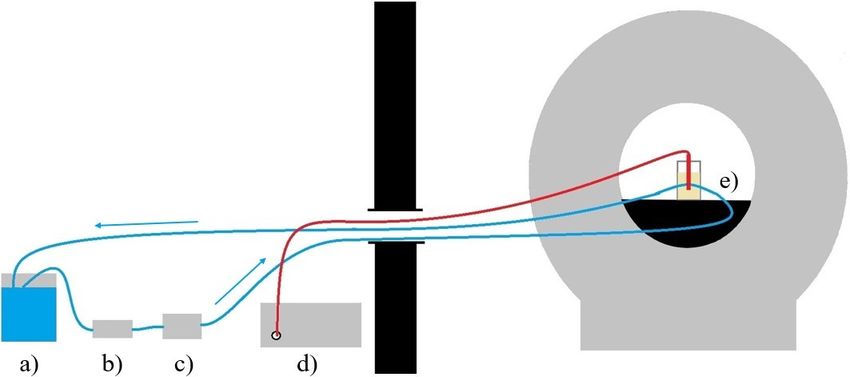
2      J. Alpers and D. Reimert et al.

use of microwave ablation (MWA). Especially for smaller tumors, MWA shows
promising results for treatment [18]. As the minimal ablative margin (MAM)
is crucial for the local tumor progression (LTP), it is of greatest importance to
assess if the malignancy has been adequately and completely treated, regardless
of the etiology. For each millimeter increase of the MAM, a 30% reduction of
the relative risk for LTP was found. The MAM is especially important as the
only significant independent predictor of LTP (p = 0.036) [8]. During the inter-
vention, magnetic resonance (MR) imaging offers several advantages like a good
soft-tissue contrast without the need of contrast agent, the free orientation and
positioning of single slice scans and the possibility to accurately track changes
in the temperature inside the tissue [5,7,14,16].

Contribution. In this work, we propose a novel approach for the creation of a
volumetric thermometry map without the development of a fully 3D sequence.
The introduced 2.5D thermometry method utilizes any common 2D gradient-
echo (GRE) sequences. Therefore, possible temporal limitations are less restrict-
ing than for the 3D sequences and images with higher resolution may be acquired
offering standard thermometry accuracy of around 1◦ C deviation while being
more robust towards MR inhomogeneities [5]. We will show that our method is
well-suited to reconstruct the actual coagulation zone after thermal ablation.

Related Work. Zhang et al.[20] propose a golden-angle-ordered 3D stack-of-
radial multi-echo spoiled gradient-echo sequence with a variable flip angle. The
image reconstruction is performed offline offering a temporal resolution between
2s-5s. Jiang et al.[6] use an accelerated 3D echo-shifted sequence and the Gad-
getron framework for image reconstruction. Temporal resolution lies at around
3s with a temperature error of less than 0.65◦ C. Quah et al.[13] are aiming at an
increased volume coverage for thermometry without multiple receive coils. An
extended k-space hybrid reconstruction was used, yielding an error of < 1◦ C and
an acquisition time of 3.5s for each image. Fielden et al.[3] present a comparison
study between cartesian, spiral-out and retraced spiral-in/out (RIO) trajecto-
ries. Using the 3D RIO sequence, they achieved a true temporal resolution of
5.8s with a temporal standard deviation of 1.32◦ C. Marx et al.[10] introduced
the MASTER sequence for volumetric MR thermometry acquisition, acquiring
six slices in around 5s. In a later work [9] they use optimized multiple-echo spi-
ral thermometry sequences, which yield a better precision than the usual 2D
Fourier transform thermometry. Image acquisition takes between 7s-11s. Svedin
et al.[17] make use of a multi-echo pseudo-golden angle stack-of-stars sequence
and offline image reconstruction using MATLAB. They achieved a temporal res-
olution of around 2s and a spatial average of the standard deviation through a
time of 0.3 − 1.0◦ C. Odéen et al.[12] propose the use of a 3D gradient recalled
echo pulse sequence with segmented EPI readout. To estimate the temperature
change, they also integrate a bioheat equation. They achieved a temperature
root mean square error of 1.1◦ C. Golkar et al.[4] introduce a fast GPU based
simulation approach for cryoablation monitoring. The reconstruction takes 110s
2.5D Thermometry Maps for MRI-guided Tumor Ablation            3

and the final result shows a Dice coefficient of 0.82. A summarize of the related
work in comparison to our method is shown in Table 1.

Table 1. Overview about the related work in comparison to this work. Every work has
been observed according to the following: 1) The kind of image sequence used. 2) The
online or offline capability of the reconstruction framework. 3) The temporal resolution
of the whole image acquisition in seconds. 4) The temperature accuracy in °C. 5) The
resulting Dice Score similarity measurement if available.

                         Image    Reconstruction Temporal Temperature
                                                                           Dice Score
                       Sequence     Framework Resolution [s] Accuracy [°C]
 Zhang et al.[20]         3D          offline      2-5            —            —
                                      online
    Jiang et al.[6]       3D                         3
4 J. Alpers and D. Reimert et al.
date 2D thermometry map for the current orientation during the treatment. To
do so, the proton resonance frequency shift (PRFS) method is used as described
by Rieke et al. [14]. The temperature T based on the PRFS is computed using
the following Equation
φ(t) − φ(t0 )
T = + T0 (1)
γαB0 T E
with φ(t)−φ(t0 ) defining the phase difference between the current time point φ(i)
and the reference timepoint φ(i0 ), γ = 42, 576 MTHz representing the gyromag-
netic ratio of hydrogen protons, α = 0.01 ppm
∆T representing the proton resonance
frequency change coefficient, B0 representing the used magnetic field strength
and T E representing the used echo time. The constant T0 needs to be added
to the temperature since Equation 1 otherwise only computes the temperature
change, neglecting the tissue’s base temperature. The Access-I integration and
2D thermometry computation were implemented as modules using MeVisLab
3.4.1 [15]. The 2.5D thermometry reconstruction itself was implemented using
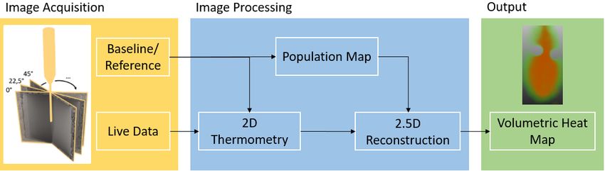
Fig. 1. Schematic overview of the proposed method.
C++. A schematic overview of the method can be seen in Figure 1. To handle
the voxel values during slice rotation every cartesian coordinate was mapped to
the corresponding cylindrical coordinate representation using Equation 2,
Pr (x, y, z) = Pc (r, θ, z) (2)
q
2 2
r = (x − xc ) + (y − yc )
x − xc
θ = atan2
y − yc
where x, y represents the Cartesian coordinates of the current voxel and xc , yc
represents the Cartesian coordinates of the centerline corresponding to the appli-
cator’s axis for every slice z in the reconstructed volume. Upon acquisition of the
reference images, a multi-dimensional population map is created. For each voxel
(xi , yi , zi ) in the reconstructed volume, this population map holds information
about the radius r and angle θ of the cylindrical coordinates, the general inter-
polation weight Iw , the adjacent interpolation partner coordinates IPlef t (x, y)2.5D Thermometry Maps for MRI-guided Tumor Ablation 5
and IPright (x, y) in the 2D live data as Cartesian representation and the weights
w1 and w2 of those interpolation partners. The weights may be acquired using
Equation 3,
θIPlef t − θi
w1 = (3)
θIPlef t − θIPright
w2 = 1 − w1
with θi representing the cylindric angle of the current Voxel i and θIPlef t , θIPright
representing the orientation angles of the left and right interpolation partners,
respectively. The 2D population map can be applied to every slice of the final
3D output volume, reducing the computational power needed. During the inter-
vention, every acquired live image triggers the reconstruction of the up-to-date
2.5D thermometry map. Here, the heat value for each voxel is reconstructed
using Equation 4,
Ti = Iw · (w1 · TIPlef t + w2 · TIPright ) (4)
with Ti representing the temperature of the current voxel i and TIPlef t , TIPright
representing the temperature of the adjacent interpolation partners. Occurring
vessels or other structures, which cause a heat sink effect are segmented during
the intervention planning. Subsequently, the segmented structure is saved as an
additional Look-Up Volume. Here, each voxel can be checked if it is part of a
heat sink structure. Using this knowledge, the interpolation weight Iw , which
ranges between [0, 1], may be adjusted. Figure 2 shows a single dimension of
the population map for parameter weighting, a reconstructed heat map, a co-
agulation estimation based on an empirically defined threshold and the corre-
sponding ground truth segmentation. The source code is available for download
at https://github.com/jalpers/2.5DThermometryReconstruction.
2.3 Evaluation
Phantom design. To create a first proof of concept, a pilot study was conducted
to evaluate the 2.5D thermometry reconstruction using 13 bio protein phantoms
as described by Bu Lin et al.[2]. The coagulation zone’s visibility in the post-
treatment data sets increased by adding a contrast agent (0, 5µmol/L Dotarem)
to the phantoms. For six phantoms, additional polyvinyl chloride (PVC) tubes
with a diameter of 5mm and a wall thickness of 1mm were integrated into the
phantoms (three single-tubes, three double-tubes) to simulate a possible heat
sink (HS) effect.
Experimental setup. The applicator of the permittivity feedback control MWA
system (MedWaves Avecure, Medwaves, San Diego, CA, USA, 14G) was placed
inside the phantom by sight and secured in position. Subsequently, the phan-
toms were placed inside a 1, 5T MR scanner (Siemens Avanto, Siemens Health-
ineers, Germany). The coaxial cables connected to the applicator and MW gen-
erator were led through a waveguide. Chokes and electrical grounding mea-
sures were added as described by Gorny et al.[5] to reduce radio frequency6 J. Alpers and D. Reimert et al.
Fig. 2. A) Example population map for output weights color coded on gray scale. B)
Reconstructed volumetric heat map. C) Estimated coagulation necrosis based on a
threshold of 57◦ C. D) Manually segmented ground truth.
interference. In the case of the perfusion phantoms, the PVC tubes were led
through the wave guide. They were connected to a diaphragm pump and a
water reservoir outside the scanning room. A flow meter (SM6000, ifm elec-
tronic, Essen, Germany) was interposed between the reservoir and the pump,
providing a flow rate of 800mL/min. Observations showed a moderate HS effect
using this setup with a maximum antenna power of 36W. Additionally, tem-
perature sensors were inserted in two phantoms to experimentally verify the
temperature accuracy of 1◦ C. Right before treatment, ten reference phase im-
ages were acquired and averaged for each orientation to compensate for static
noise. The MWA duration was set to 15 minutes with a temperature limit of
90◦ C. The GRE sequence offers a slice thickness of 5mm, a field of view (FOV)
of 256mm ∗ 256mm, a matrix of 256 ∗ 256, and a bandwidth of 260Hz/P x.
Image acquisition took around 1.1s with a 5s break to simulate the temporal
resolution for a breathing patient. The TE was 3.69ms, the TR 7.5ms, and the
flip angle 7◦ . For post-treatment observation a 3D turbo spin echo (TSE) se-
quence (TE = 156ms, TR = 11780ms, flip angle = 180◦ , matrix = 256 ∗ 256,
FOV = 256mm ∗ 256mm, bandwidth = 40Hz/P x, slice thickness = 1mm)
was used. The 3D TSE allows for proper visualization of the real coagulation
zone due to a very high tissue contrast. Extraction of the coagulation ground
truth was done manually by a clinical expert using MEVIS draw (Fraunhofer
MEVIS, Bremen, Germany). All data sets used are available for download at
http://open-science.ub.ovgu.de/xmlui/handle/684882692/89.
Statistical evaluation. Final evaluation of the acquired data was performed
using the dice similarity coefficient (DSC) as explained in Equation 5
2 ∗ TP
DSC = (5)
2 ∗ TP + FP + FN2.5D Thermometry Maps for MRI-guided Tumor Ablation 7
Fig. 3. Experimental evaluation setup. Flexible tubes (blue) lead the water (a) through
a flow meter (b), a diaphragm pump (c) and the bio protein phantom (e). The coaxial
cables (red) connect the applicator with the MW generator d).
with T P representing the true positives, F P the false positives and F N the false
negatives. Additionally, the standard error of the mean (SEM) was computed at
a confidence level of 95% (p = 0.05) using Equation 6
rP
(xi − x̄)2
σ= (6)
N −1
σ
SEM = √ ∗ 1.96
N
with σ representing the standard deviation, xi the current sample, x̄ the mean
value and N the sample size. To compute the SEM at a confidence level of 95%
it has to be multiplied by 1.96, which is the approximated value of the 97.5
percentile of the standard normal distribution.
3 Results
Summarized evaluation results can be seen in Figure 4. Empirically determined
coagulation thresholds were set between 51◦ C and 61◦ C depending on each phan-
tom’s pH value. It is noticeable that the DSCs for HS phantoms show a very
high SEM with 0.70 ± 0.15(±21.25%) and 0.74 ± 0.06(±8.49%) regarding the
sensitivity. The high range results from a corrupted dataset due to heavy ar-
tifacts within the image data. Leaving the corrupted dataset out of the evalu-
ation, the SEM shows a significantly lower deviation of 0.76 ± 0.062(±8.07%)
and 0.77±0.048(±6.25%) for the DSC and sensitivity, respectively. Observations
show a slightly higher DSC and sensitivity for phantoms without any HS effect.
Here, the values range from 0.79±0.04(±4.53%) and 0.79±0.04(±5.55%), respec-
tively. Evaluation showed an overall SEM for the DSC of 0.75 ± 0.07(±9.76%)8 J. Alpers and D. Reimert et al. Fig. 4. Summarized evaluation results for phantoms without HS effect, phantoms with HS effect and the overall results. Note that the data range [0,0.3] was left out because no data points are present in that range. and a SEM for sensitivity of 0.77 ± 0.04(±4.99%). To evaluate the computa- tional effort, every major step was performed 100 times. The creation of the population map and the heat sink look up volume took 25.53ms ± 3.33ms and 3.91s ± 0.59s, respectively. These two steps need to be done just once before start of the treatment. The reconstruction of the 2.5D thermometry map was performed in 18.02ms±5.91ms on a customary workstation (Intel( R) Core(TM) i5-6200U CPU, double-core 2.30GHz, 8GB RAM, Intel(R) HD Graphics 520). This reconstruction will be performed every time a new image is acquired during treatment. 4 Discussion and Conclusion The aim of this work is to develop a volumetric thermometry map, which can be applied to a wide variety of clinical setups. Therefore, our work heavily re- lies on the up-to-date standard 2D GRE sequence for image acquisition. This allows for the standard accuracy of the thermometry up to 1.0◦ C. Nonetheless, the sampling of the 3D volume also results in some disadvantages, which need to be addressed in the future. First, the diffusion of the heat inside the tissue is not linear over time. Therefore, it would be necessary to include an adaptive temporal and spatial resolution depending on the current intervention time. A new study should be conducted to identify an optimal sequence protocol for this 2.5D thermometry approach. Second, we found that the reconstruction some- times shows stair-case artifacts. Because only one image is acquired every few seconds, the time difference between adjacent orientations may be very high. The temperature difference for each voxel dependent on the applicator’s radius
2.5D Thermometry Maps for MRI-guided Tumor Ablation              9

may be computed and applied to the corresponding voxel on every other out-of-
date data to compensate for this error. This transfer of the heat gradient may
improve the reconstruction accuracy. Another approach may be the use of a
model-based reconstruction to take different tissue characteristics into account.
To pseudo-increase the temporal resolution, bio heat transfer simulations may
also be included during reconstruction. The acquired live data may be able to
adjust the simulation parameters to increase the simulation accuracy. Finally,
our study only performs on bio protein phantoms. Results show a proof of con-
cept for the proposed method, but it still has to be evaluated in real tissue and
a more realistic clinical environment. Therefore, perfused ex vivo livers may be
a way to go in the future. Additionally, we currently assume a breath-holding
state or at least a breath-triggered image acquisition. Research shows that a
wide range of interventional registration methods is available, but further inves-
tigations in this area still need to be done to create an applicable method. The
last issues arise because of the MR inhomogeneity during image acquisition. The
slightest disturbances may result in heavy image artifacts. Proper shielding of
the MW generator is needed to reduce the SNR loss over time thus increasing
the thermometry and reconstruction accuracy.

In conclusion, we proposed a novel method for 2.5D thermometry map recon-
struction based on common GRE sequences rotated around the applicator’s main
axis. A pilot study was conducted using bio protein phantoms to simulate cases
with possible heat sink effects and without. The evaluation shows promising
results regarding the DSC of the reconstructed 2.5D thermometry map and a
manually defined ground truth. Future work should address the reconstruction
method’s improvement by integrating further apriori knowledge like the esti-
mated shape of the heat distribution. Furthermore, a more realistic study should
be conducted with bigger sample size and real tissue. In sum, the method shows
a high potential to improve the clinical success rate of minimally invasive abla-
tion procedures without necessarily hampering the standard clinical workflow of
the individual clinician.

References
 1. Ahmed, M., Solbiati, L., Brace, C.L., Breen, D.J., Callstrom, M.R., Charboneau,
    J.W., Chen, M.H., Choi, B.I., de Baère, T., Dodd III, G.D., et al.: Image-guided
    tumor ablation: standardization of terminology and reporting criteria—a 10-year
    update. Radiology 273(1), 241–260 (2014)
 2. Bu-Lin, Z., Bing, H., Sheng-Li, K., Huang, Y., Rong, W., Jia, L.: A polyacrylamide
    gel phantom for radiofrequency ablation. International Journal of Hyperthermia
    24(7), 568–576 (2008)
 3. Fielden, S.W., Feng, X., Zhao, L., Miller, G.W., Geeslin, M., Dallapiazza, R.F.,
    Elias, W.J., Wintermark, M., Butts Pauly, K., Meyer, C.H.: A spiral-based volu-
    metric acquisition for MR temperature imaging. Magnetic resonance in medicine
    79(6), 3122–3127 (2018)
 4. Golkar, E., Rao, P.P., Joskowicz, L., Gangi, A., Essert, C.: Fast gpu computation
    of 3d isothermal volumes in the vicinity of major blood vessels for multiprobe
10 J. Alpers and D. Reimert et al.
cryoablation simulation. In: International Conference on Medical Image Computing
and Computer-Assisted Intervention. pp. 230–237. Springer (2018)
5. Gorny, K.R., Favazza, C.P., Lu, A., Felmlee, J.P., Hangiandreou, N.J., Browne,
J.E., Stenzel, W.S., Muggli, J.L., Anderson, AG, Thompson, S.M., et al.: Practical
implementation of robust MR-thermometry during clinical MR-guided microwave
ablations in the liver at 1.5 T. Physica Medica 67, 91–99 (2019)
6. Jiang, R., Jia, S., Qiao, Y., Chen, Q., Wen, J., Liang, D., Liu, X., Zheng, H., Zou,
C.: Real-time volumetric MR thermometry using 3D echo-shifted sequence under
an open source reconstruction platform. Magnetic resonance imaging 70, 22–28
(2020)
7. Kägebein, U., Speck, O., Wacker, F., Hensen, B.: Motion correction in proton res-
onance frequency–based thermometry in the liver. Topics in Magnetic Resonance
Imaging 27(1), 53–61 (2018)
8. Laimer, G., Schullian, P., Jaschke, N., Putzer, D., Eberle, G., Alzaga, A., Odisio,
B., Bale, R.: Minimal ablative margin (mam) assessment with image fusion: an
independent predictor for local tumor progression in hepatocellular carcinoma after
stereotactic radiofrequency ablation. European radiology 30(5), 2463–2472 (2020)
9. Marx, M., Ghanouni, P., Butts Pauly, K.: Specialized volumetric thermometry for
improved guidance of MR g FUS in brain. Magnetic resonance in medicine 78(2),
508–517 (2017)
10. Marx, M., Plata, J., Pauly, K.B.: Toward volumetric MR thermometry with the
MASTER sequence. IEEE transactions on medical imaging 34(1), 148–155 (2014)
11. Mauri, G., Sconfienza, L.M., Pescatori, L.C., Fedeli, M.P., Alı̀, M., Di Leo, G., Sar-
danelli, F.: Technical success, technique efficacy and complications of minimally-
invasive imaging-guided percutaneous ablation procedures of breast cancer: a sys-
tematic review and meta-analysis. European radiology 27(8), 3199–3210 (2017)
12. Odéen, H., Almquist, S., de Bever, J., Christensen, D.A., Parker, D.L.: Mr ther-
mometry for focused ultrasound monitoring utilizing model predictive filtering and
ultrasound beam modeling. Journal of therapeutic ultrasound 4(1), 1–13 (2016)
13. Quah, K., Poorman, M.E., Allen, S.P., Grissom, W.A.: Simultaneous multislice
mri thermometry with a single coil using incoherent blipped-controlled aliasing.
Magnetic resonance in medicine 83(2), 479–491 (2020)
14. Rieke, V., Butts Pauly, K.: MR thermometry. Journal of Magnetic Resonance
Imaging: An Official Journal of the International Society for Magnetic Resonance
in Medicine 27(2), 376–390 (2008)
15. Ritter, F., Boskamp, T., Homeyer, A., Laue, H., Schwier, M., Link, F., Peitgen,
H.O.: Medical image analysis. IEEE pulse 2(6), 60–70 (2011)
16. de Senneville, B.D., Mougenot, C., Quesson, B., Dragonu, I., Grenier, N., Moo-
nen, C.T.W.: MR thermometry for monitoring tumor ablation. European radiology
17(9), 2401–2410 (2007)
17. Svedin, B.T., Payne, A., Bolster Jr, B.D., Parker, D.L.: Multiecho pseudo-golden
angle stack of stars thermometry with high spatial and temporal resolution using
k-space weighted image contrast. Magnetic resonance in medicine 79(3), 1407–1419
(2018)
18. Tehrani, M.H., Soltani, M., Kashkooli, F.M., Raahemifar, K.: Use of microwave
ablation for thermal treatment of solid tumors with different shapes and sizes—a
computational approach. Plos one 15(6), e0233219 (2020)
19. Tomasian, A., Gangi, A., Wallace, A.N., Jennings, J.W.: Percutaneous thermal
ablation of spinal metastases: recent advances and review. American Journal of
Roentgenology 210(1), 142–152 (2018)2.5D Thermometry Maps for MRI-guided Tumor Ablation 11
20. Zhang, L., Armstrong, T., Li, X., Wu, H.H.: A variable flip angle golden-angle-
ordered 3d stack-of-radial mri technique for simultaneous proton resonant fre-
quency shift and t1-based thermometry. Magnetic resonance in medicine 82(6),
2062–2076 (2019)You can also read