ADAPTIVE AUTOMOTIVE RADAR DATA ACQUISITION - OpenReview
←
→
Page content transcription
If your browser does not render page correctly, please read the page content below
Under review as a conference paper at ICLR 2021

A DAPTIVE AUTOMOTIVE R ADAR DATA ACQUISITION
 Anonymous authors
 Paper under double-blind review

                                           A BSTRACT

        In an autonomous driving scenario, it is vital to acquire and efficiently process data
        from various sensors to obtain a complete and robust perspective of the surround-
        ings. Many studies have shown the importance of having radar data in addition to
        images since radar improves object detection performance. We develop a novel
        algorithm motivated by the hypothesis that with a limited sampling budget, al-
        locating more sampling budget to areas with the object as opposed to a uniform
        sampling budget ultimately improves relevant object detection and classification.
        In order to identify the areas with objects, we develop an algorithm to process
        the object detection results from the Faster R-CNN object detection algorithm and
        the previous radar frame and use these as prior information to adaptively allocate
        more bits to areas in the scene that may contain relevant objects. We use previ-
        ous radar frame information to mitigate the potential information loss of an object
        missed by the image or the object detection network. Also, in our algorithm, the
        error of missing relevant information in the current frame due to the limited bud-
        get sampling of the previous radar frame did not propagate across frames. We
        also develop an end-to-end transformer-based 2D object detection network using
        the NuScenes radar and image data. Finally, we compare the performance of our
        algorithm against that of standard CS and adaptive CS using radar on the Oxford
        Radar RobotCar dataset.

1   I NTRODUCTION

The intervention of deep learning and computer vision techniques for autonomous driving scenario
is aiding in the development of robust and safe autonomous driving systems. Similar to humans
navigating their world with numerous sensors and information, the autonomous driving systems
need to process different sensor information efficiently to obtain the complete perspective of the
environment to safely maneuver. Numerous studies Meyer & Kuschk (2019), Chang et al. (2020)
have shown the importance of having radar data in addition to images for improved object detection
performance. The real-time radar data acquisition using compressed sensing is a well-studied field
where, even with sub-Nyquist sampling rates, the original data can be reconstructed accurately.
During the onboard signal acquisition and processing, compressed sensing will reduce the required
measurements, therefore, gaining speed and power savings. In adaptive block-based compressed
sensing, based on prior information with a limited sampling budget, radar blocks with objects would
be allocated more sampling resources while maintaining the overall sampling budget. This method
would further enhance the quality of reconstructed data by focusing on the important regions. In
our work, we split the radar into 8 azimuth blocks and used the 2D object detection results from
images as prior data to choose the important regions. The 2D object detection network generates
the bounding boxes and object classes for objects in the image. The bounding boxes were used to
identify the azimuth of the object in radar coordinates. This helped in determining the important
azimuth blocks. As a second step, we used both previous radar information and the 2-D object
detection network to determine the important regions and dynamically allocate the sampling budget.
The use of previous radar data in addition to object information from images mitigates the loss of
object information either by image or the object detection network.
Finally, we have also developed an end-to-end transformer-based 2-D object detection Carion et al.
(2020) network using the NuScenes Caesar et al. (2020) radar and image dataset. The object detec-
tion performance of the model using both Image and Radar data performed better than the object
detection model trained only on the image data.

                                                  1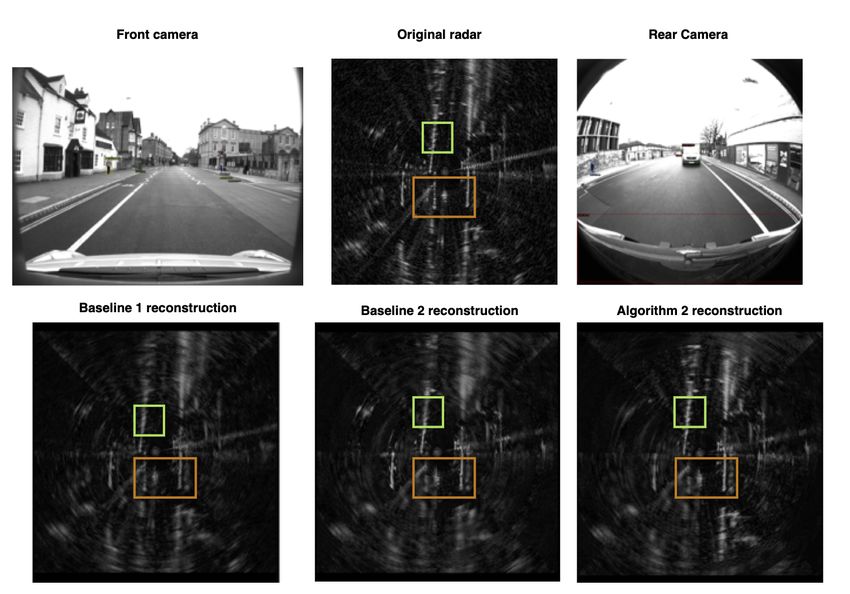
Under review as a conference paper at ICLR 2021

Our main contributions are listed below:

       • We have developed an algorithm in a limited sampling budget environment to dynamically
         allocate more sampling budget to important radar return regions based on the prior im-
         age data processed by the Faster R-CNN object detection network Ren et al. (2015) while
         maintaining the overall sampling budget.
       • In the extended algorithm, important radar return regions are selected using both object
         detection output and the previous radar frame.
       • We’ve designed an end-to-end transformer-based 2-D object detection network (DETR-
         Radar) Carion et al. (2020) using both Nuscenes Caesar et al. (2020) radar and image data.

2   R ELATED WORK

The compressed sensing technique is a well-studied method for sub-Nyquist signal acquisition. In
Roos et al. (2018), they showed the successful application of standard compressed sensing on radar
data with 40% sampling rate. They also showed that they could use a single A/D converter for
multiple antennas. In our method, we have shown efficient reconstruction with 10% sampling rate.
In another work, Slavik et al. (2016), they used standard compressed sensing-based signal acquisi-
tion for noise radar with 30% sampling rate. Whereas, we’ve developed this algorithm for FMCW
scanning radar. Correas-Serrano & González-Huici (2018) analyzed various compressed sensing
reconstruction algorithms such as Orthogonal Matching Pursuit (OMP), Basis Pursuit De-noising
(BPDN) and showed that, in automotive settings, OMP performs better reconstruction than the other
algorithms. In our algorithm, we have used Basis Pursuit(BP) algorithm for signal reconstruction
because, although it is computationally expensive than OMP, BP requires fewer measurements for
reconstruction Sahoo & Makur (2015).
The Adaptive compressed sensing technique was used for radar acquisition by Assem et al. (2016).
They used the previously received pulse interval as prior information for the present interval to de-
termine the important regions of the pulsed radar. In our first algorithm, we used only the image data
and in the second algorithm, we used both image and previous radar data on the FMCW scanning
radar. In another work, Kyriakides (2011) they used adaptive compressed sensing for a static tracker
case and have shown improved target tracking performance. However, in our algorithm, we’ve used
adaptive compressed sensing for radar acquisition from an autonomous vehicle where, both the ve-
hicle and the objects were moving. In Zhang et al. (2012) they used adaptive compressed sensing
by optimizing the measurement matrix as a separate least squares problem, in which only the targets
are moving. This increases the computational complexity of the overall algorithm. Whereas in our
method, the measurement matrix size is increased to accommodate more sampling budget which has
the same complexity as the original CS measurement matrix generation technique. In a separate but
related work, Nguyen et al. (2019) LiDAR data was acquired based on Region-of-Interest derived
from image segmentation results of images. In our work, we acquired radar data using 2-D object
detection results.
Apart from radar, adaptive CS was used for images and videos. In Mehmood et al. (2017), the
spatial entropy of the image helped in determining the important regions. The important regions
were then allocated more sampling budget than the rest which improved reconstruction quality. In
another work, Zhu et al. (2014), the important blocks were determined based on the variance of
each block, the entropy of each block and the number of significant Discrete Cosine Transform
(DCT) coefficients in the transform domain. In Wells & Chatterjee (2018), object tracking across
frames of a video was preformed using Adaptive CS. The background and foreground segmentation
helped in allocating higher sampling density to the foreground and very low sampling density to
the background region. Liu et al. (2011) similarly used adaptive CS for video acquisition based on
inter-frame correlation. Also, Ding et al. (2015), performed the joint CS of two adjacent frames in a
video based on the correlation between the frames.
Finally, numerous studies showed the advantage of using both radar and images in an object de-
tection network for improved object detection performance. Nabati & Qi (2019) used radar points
to generate region proposals for the Fast R-CNN object detection network which made the model
faster than the selective search based region proposal algorithm in Fast R-CNN. Nobis et al. (2019),
Chadwick et al. (2019) showed that radar in addition to image improved distant vehicle object detec-

                                                  2
Under review as a conference paper at ICLR 2021 tion and occluded object detection due to adverse weather conditions. In Chang et al. (2020), spatial attention was used to combine radar and image features for improved object detection using FCOS Tian et al. (2019) object detection network. 3 M ETHOD 3.1 DATASET The Oxford Radar RobotCar dataset Barnes et al. (2019) consists of various sensor readings while the vehicle was driven around Oxford, the UK in January 2019. The vehicle was driven for a total of 280km in an urban driving scenario. We have used camera information from the center captured with Point Grey Bumblebee XB3 at 16 Hz, rear data captured by Point Grey Grasshopper2 at 17 Hz. The Radar data was collected by NavTech CT350-X, Frequency Modulated Continuous-Wave scanning radar with 4.38 cm range resolution and 0.9 degrees in rotation resolution at 4 Hz. They captured radar data with a total range of 163m. In addition to this, they have released the ground- truth radar odometry. However, in our case, we require 2D object annotation on the radar data to validate our approach. Since this a labor-intensive task, we chose 3 random scenes from the Oxford dataset, each with 10 to 11 radar frames and marked the presence or absence of the target object across reconstructions. To the best of our knowledge, this is the only publicly available raw radar dataset. Hence, we used this dataset for testing our compressed sensing algorithm. In order to train our DETR-Radar object detection model, we used the NuScenes v0.1 dataset Caesar et al. (2020). This is one of the publicly available datasets for autonomous driving with a range of sensors such as Cameras, LiDAR and radar with 3D bounding boxes. Similar to Nabati & Qi (2019), we have converted all the 3D bounding box annotations to 2D bounding boxes and merged similar classes to 6 total classes, Car, Truck, Motorcycle, Person, Bus and Bicycle. This dataset consists of around 45k images and we have split the dataset into 85% training and 15% validation. 3.2 A DAPTIVE B LOCK -BASED C OMPRESSED S ENSING Compressed Sensing is a technique where, if the original signal x, with x 2 RN , the measurement y is taken using the measurement matrix , using y = x, where, 2 R(M XN ) and y 2 RM with an effective number of measurements, M
Under review as a conference paper at ICLR 2021

Figure 1: The overview of Algorithm 1 and Algorithm 2. Algorithm 1 takes front and rear camera
data as input to identify the important azimuth blocks. Algorithm 2 samples radar data based on
azimuth from images and the previous radar frame.

images, in this case, we can only choose azimuth sections and not the range. The chosen sections
were dynamically allocated more sampling rate than the others. Also, since the radar data was
acquired with 163 m range, we allocated more sampling rate to the first 18 range blocks compared
to the last 19 since there is not much useful information in the farther range values. The average
driving speed in an urban environment is 40 miles per hour. Since radar is captured at 4 Hz, for every
frame, the object could have moved 4.25m. Since the bin resolution is 4.38cm and for a particular
block with 100 bins, the area spanned would be 4.38m. Since we are looking into the first 18 range
blocks, that covers a total area of 78.84m. Hence, in an urban setting, the moving vehicle can be
comfortably captured by focusing within the 78.84m range. In a freeway case, for an average speed
of 65 miles per hour, the vehicle could have moved 7.2m per frame and again, this would be captured
by focusing on the first 78.84m. Algorithm 1 steps:

      1. Acquire front and rear camera information at t=0s.
      2. Process them simultaneously through the Faster R-CNN network and generate results at
         t=0.12s.
      3. Process the Faster R-CNN results to determine the important azimuth blocks for radar.
      4. Dynamically allocate more sampling rate to the chosen azimuth blocks and fewer to the
         other blocks while maintaining the total sampling budget.
      5. Acquire the radar data at t=0.25s based on the recommenced sampling rate.

3.4   A LGORITHM 2

However, in order to avoid the effects of the blind spot region of the camera, the lost information
from the camera due to weather or other effects and object missed by the object detection network,

                                                  4
Under review as a conference paper at ICLR 2021
we designed the extended algorithm to utilize the previous radar information to sample the current
radar frame, in addition, to object detection results from images. In order to maintain the bit bud-
get, the chosen range blocks for a particular azimuth is further limited to 14, covering 61.32m in
range. Based on the speed of the vehicle explanation given in the algorithm 1 section for urban and
freeway environment, the moving vehicles can still be captured within the 61.32m range from the
autonomous vehicle. Therefore, the balance sampling budget is used to provide a higher sampling
rate to the chosen blocks from algorithm 2. Algorithm 2 steps:
1. Repeat steps 1 to 5 from algorithm 1 for frame 1.
2. Repeat steps 1 to 3 from algorithm 1.
3. Using the Constant False Alarm Rate (CFAR) Richards (2005) detection algorithm, the
blocks with point clouds from radar data are additionally chosen to have a higher sampling
rate.
4. Acquire the radar data based on the above allocation.
As shown in figure 1, Algorithm 1 takes rear and front camera images and predicts object class
and bounding boxes. The object’s x coordinate in the front camera image is converted from the
cartesian plane to azimuth ranging from -33 to 33 degrees corresponding to the HFoV of the front
camera. The object’s x coordinate from the rear camera is converted to azimuth ranging from 90
to 270 degrees. Therefore, if an object is present in one of the 8 azimuth blocks, divided as 0-45
degrees, 45-90 degrees and so on, that azimuth block is considered important and allocated more
sampling rate. Algorithm 2 is an extension of Algorithm 1, in addition to azimuth, if a radar point
cloud is detected in any of the blocks (50x100), they are marked necessary and were allocated more
sampling rate. In the experiments section, we have shown cases where the radar point clouds helped
in identifying objects present in the camera’s blind spot.
3.5 DETR-R ADAR
The Faster R-CNN Ren et al. (2015) object detection network is one of the well-refined techniques
for 2D object detection. However, it relies heavily on two components, non-maximum suppression
and anchor generation. The end-to-end transformer-based 2D object detection introduced in Carion
et al. (2020), eliminates the need for these components. We included radar data in two ways. In the
first case, we included the radar data as an additional channel to the image data Nobis et al. (2019).
In the second case, we rendered the radar data on the image. We used perspective transformation
based on Nabati & Qi (2019) to transform radar data points from the vehicle coordinates system
to camera-view coordinates. The models where radar data were included as an additional channel
were trained for a longer duration since the first layer of the backbone structure had to be changed
to accommodate the additional channel. In all the above cases, the models were pre-trained on the
COCO dataset and we fine-tuned them on the NuScenes data. To the best of our knowledge, we are
the first ones to implement end-to-end transformer-based 2D object detection using both image and
radar data.
4 E XPERIMENTS
In order the validate our approach, we tested it on 3 scenes from the Oxford radar robot car dataset.
The image data were processed using the Faster R-CNN object detection network Girshick et al.
(2018) to obtain object classes and 2D bounding boxes. ResNet-101 was used as the backbone
structure, which was pre-trained on the ImageNet dataset Russakovsky et al. (2015). The faster R-
CNN network was trained on the COCO train dataset and gave 39.8 box AP on the COCO validation
dataset. Since the model was originally trained on the COCO dataset, it predicts 80 classes. How-
ever, we filtered pedestrians, bicycle, car and truck classes from the predictions for a given scene.
In order to capture and present the radar data clearly, we have shown data for a range of 62.625m
from the autonomous vehicle. Although the original radar data is captured for a range of 163m, we
could find meaningful information in the first 62.625m. The total sampling budget was set to 10%.
Therefore, baseline 1 reconstruction was uniformly provided with 10% sampling rate for the entire
frame and were reconstructed using standard CS. In baseline 2, similar to Assem et al. (2016), the
important blocks were determined using the pointcloud information from the previous radar frame.
5Under review as a conference paper at ICLR 2021
However, the first frame for a scene was acquired with uniform sampling of 10%. From the second
frame, if an object was detected using CFAR in the previous frame in a given block, it was deemed
essential and the sampling budget to that block was increased. We set the overall budget to 10%
and all the non-important blocks had 5% sampling rate. Therefore, the remaining sampling rate was
equally distributed to all the important blocks as suggested by the CFAR algorithm.
In algorithm 1, we split the radar into three regions. R1: The chosen azimuth until 18th range block
(78.84m), R2: the other azimuth regions until the 18th range block (78.84m) and finally, R3: all the
azimuth blocks from 19th to 37th range block. Since the object detection on image data does not
provide the depth information, for a particular chosen azimuth block, we will be forced to choose
the entire range of 163m. However, in the urban and freeway scenario, as explained in the methods
sections, the moving vehicle can be comfortably captured within the first 18 blocks (78.84m) and
hence we chose the first 18 blocks as the R1 region. The purpose of splitting the regions into R1, R2
and R3 is to provide with decreasing sampling rate based on decreasing importance. Moreover, the
regions could have been split as 16 blocks as in the case of Algorithm 2 or 20 blocks as well which
would have only changed the sampling rate allocation to different regions. Since across different
scenes, there could have been a variable number of important azimuth blocks, if the chosen azimuth
block was less than 50% i.e., less than 4 out of 8, we randomly sampled more azimuth blocks. Also,
if it was more than 4, we avoided losing important information by reducing the sampling rate in the
R1 region. We fixed the sampling rate for R2 and R3 initially. R3 had the lowest sampling rate of
2.5% because it covered the region around the autonomous vehicle that was 78.84m away. Similarly,
R2 was closer to the vehicle but based on the image information, it did not have an object and hence
we fixed the sampling rate to 5%. Therefore, based on the number of important azimuth blocks, we
solved for the sampling rate of R1. Hence, when there were 4 azimuth blocks, R1 was sampled at
30.8%, R2 at 5% and R3 at 2.5% sampling rate. In the case of 5 azimuth blocks, R1 was sampled at
25.5%, R2 and R3 at 5% and 2.5% respectively. In the case of 6 azimuths, R1 at 20.2%, R2 at 5%
and R3 at 2.5%.
In algorithm 2, again, the regions were again split into 3. However, R1: The chosen azimuth until
14th range (61.32m), R2 was the other azimuth region until 14th and R3 were from 15th to 37th range
block. In this case, we retained the sampling rate across regions from algorithm 1. But, we reduced
the number of blocks in the R1 region from 18 to 14. Again, although we reduced the R1 region
to the first 61.32m, the moving vehicle can be comfortably captured based on the explanation from
methods. The previous reconstructed radar frame was processed by the CFAR detector to identify
point clouds corresponding to objects. If a radar block had a point cloud, it was deemed important.
The sampling budget saved from R1 was used to sample radar blocks classified as important from
the previous radar frame. In table 1, we have discussed the presence or absence/faint visibility of
an object in a frame across reconstructions. Apart from that, in all frames across scenes except
for frame 2, scene 3 truck reconstruction, the mentioned objects were sharper in our reconstruction
compared to the baseline 1. The radar images have been enhanced for better visibility of the objects.
Due to the non-availability of object annotation from the Oxford radar dataset, we had to annotate
the presence or absence of the object manually and have provided a subjective evaluation.
In the first scene, the autonomous vehicle moved across an almost straight street without turning.
There was a vehicle behind it and pedestrians on the right sidewalk and a pedestrian on the left
sidewalk to the front. As shown in the table 1, the person on the top left is not visible or very faint
on both the baseline reconstructions on frame 2 to 6. In frame 7 to 10, the person on the top left was
reconstructed by baseline 2 while it was very faint in baseline 1 reconstruction. However, the person
is visible on both the Algorithm 1 and Algorithm 2 reconstructions. In frame 2, the pedestrians on
the right side happened to be in the blind spot of both the front and rear cameras. Therefore, the
reconstruction of Algorithm 1 on that segment was poor. However, that region was captured from
the previous radar frame and a higher sampling rate was allocated to the region with pedestrians
and it was reconstructed appropriately using Algorithm 2. Apart from the listed objects in the table,
the rear vehicle was, in general, sharper than baseline reconstruction in all the frames reconstructed
using Algorithm 1 and Algorithm 2.
In scene 2, the vehicle waited on the side of an intersection for a truck to pass by. This truck is
visible in all the reconstructions. In frame 2, the car was in the blind spot and it was missed by
the CFAR in the previous radar frame as well as the image. Therefore, it is visible in the baseline
1 and it was not reconstructed by our algorithm. In frames 4-6 and 8, the car to the rear right was
missed by the camera. But, it was captured in algorithm 2 and was sharper than the baseline 1
6Under review as a conference paper at ICLR 2021
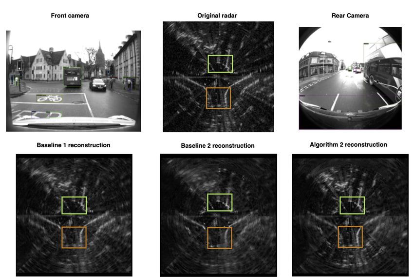
Figure 2: The figure above is from Scene 1, frame 2. In the top row, we show the front image data
and rear image processed by the 2D object detection network. The original radar corresponds to the
raw radar data acquired in the scene. The green box on the radar data, when zoomed in, would show
the person to the left on the front camera. The person is not visible on the baseline reconstructions
but can be seen in our reconstruction. The orange box highlights the truck on the rear image.
Scene Frame Object Baseline1 Baseline2 Algo1 Algo2
1 Person (top-left) no no yes -
Scene 1 2-6 Person (top-left) no no yes yes
7-10 Person (top-left) no yes yes yes
2 Pedestrians(right) yes yes no yes
7 car (top-left) no no yes yes
Scene 2 6-11 Bicycle (rear) no no yes yes
2 car (rear-right) yes no no no
4-6,8 car (rear-right) yes yes no yes
4-7 Pedestrian (rear-left) no no yes yes
9-11 Car(rear-left) yes no no yes
2-6 car (rear) no no yes yes
Scene 3
2,4 car (top-right) no yes yes yes
3 car (top-right) no no yes yes
8 car (rear-right) no no yes yes
Table 1: The table highlights the presence of an object as ’yes’ and if the object is very faint or
absent, it is indicated as ’no’.
reconstruction. Again, in frames 9-11, the car to the rear left was missed by the object detection
network. But, it was captured from the previous radar frame and it was reconstructed by Algorithm
2 with a higher sampling rate. Apart from this the car to the front of the vehicle, pedestrian at the
rear of the vehicle were reconstructed by Algorithm 1 and Algorithm 2 while it was either missed or
had a faint reconstruction by both the baseline techniques.
7Under review as a conference paper at ICLR 2021
Figure 3: The figure above is from Scene 3, frame 3. The green box when zoomed in shows the
car passing by to the right of the autonomous vehicle right below the front bus and radar returns
from the wall. The orange box highlights the car behind the autonomous vehicle, captured by our
algorithms and missed by the baselines.
In scene 3, the vehicle crossed a traffic signal. There was a bus to the left, another bus to the front
and a car passed by on the opposite direction. There were a few cars behind the vehicle. In all
the frames, the buses were captured by all the reconstruction schemes. However, our algorithm gave
sharper results than baseline 1. As shown in the table 1, the cars behind the autonomous vehicle were
captured by our algorithms. However, it was not captured by the baseline reconstructions. The result
is highlighted using an orange box in figure 3. Similarly, the car passing by on the opposite side was
captured by our algorithm and it is barely visible in the baseline reconstruction and it is highlighted
using a green box in figure 3. In raw radar, the poles and buildings tend to have a sharper appearance
than cars or pedestrians based on the size or position of the cars and pedestrians. Therefore, the car
is the tiny region right below the bus and building, highlighted by the green box. This validates the
necessity to allocate a higher sampling budget for important objects such as pedestrians or cars on
the road. Moreover, although we used previous radar information in addition to object detection
results for radar reconstruction, our algorithm did not exhibit propagation of error of missing an
object in the current frame due to poor reconstruction in the previous frame.
Finally, we trained a separate object detection network using the NuScenes image and radar data. In
this case, we limited our analysis to NuScenes image and original radar data because the Nuscenes
radar that was available to us were processed pointclouds with annotations. Whereas, the Oxford
data was the only available raw data on which we could apply CS but, without object annotations
and hence, we could not use Oxford data to train the object detection model. All of our models were
trained on the COCO detection dataset and we fine-tuned them on the Nuscenes v0.1 dataset. As
shown in the table 2, our baseline comparison is with the Nabati & Qi (2019) paper, where, they
trained the model on Nuscenes v0.1 image dataset and used the radar data for anchor generation.
The Faster R-CNN Img and Faster R-CNN RonImg models had ResNet-101 He et al. (2015) as
the backbone structure Girshick et al. (2018). The models with Img+R were trained with radar as
an additional channel. Therefore, the first layer of the backbone structure was changed to process
the additional radar channel. The DETR network Carion et al. (2020) had ResNet-50 He et al.
8Under review as a conference paper at ICLR 2021
(2015) as the backbone structure, a transformer encoder, transformer decoder followed by a 3-layer
feed-forward bounding box predictor. The main advantage of transformers is that its architectural
complexity is simpler than the Faster R-CNN and the need for Non-Maximal suppression is elimi-
nated in DETR. Also, we believe that the attention mechanism in DETR helped in focusing more on
the regions with radar points (overlapping on objects in images) and helped in better performance.
The Img and RonImg models were trained for the same number of epochs for a fair comparison.
The Img+R models were trained for additional epochs since the backbone structure’s first layer was
modified. In the Faster R-CNN case, Img+R has better performance than Img. While, in DETR,
RonImg has better performance. The Faster R-CNN Img and RonImg were trained for 25k iterations.
The Faster R-CNN Img+R was trained for 125k iterations. DETR Img and DETR RonImg models
were trained for 160 epochs. While DETR Img+R was trained for 166 epochs. The DETR - RonImg
model performed better across various metrics compared to the baseline, Faster R-CNN and DETR
Img+R model. We believe that the attention heads in the transformer architecture helped in focusing
object detection predictions around the radar points. However, the Faster R-CNN Img+R was better
than the Faster R-CNN RonImg model. We used the standard evaluation metrics, mean average
precision (AP), mean average recall (AR), average precision at 0.5, 0.75 IOU, small, medium and
large AR Lin et al. (2015).
Network AP AP50 AP75 AR ARs ARm ARl
Fast R-CNN Nabati & Qi (2019) 0.355 0.590 0.370 0.421 0.211 0.391 0.514
Faster R-CNN - Img 0.395 0.678 0.417 0.470 0.256 0.444 0.568
Faster R-CNN - Img+R 0.462 0.738 0.503 0.530 0.328 0.515 0.599
Faster R-CNN - RonImg 0.380 0.654 0.400 0.449 0.176 0.421 0.563
DETR - Img 0.471 0.802 0.504 0.616 0.384 0.572 0.725
DETR - RonImg 0.486 0.804 0.527 0.636 0.401 0.602 0.731
DETR - Img+R 0.448 0.763 0.468 0.582 0.297 0.549 0.688
Table 2: Img denotes model trained on Images, Img + R indicated model trained with Radar as an
additional channel and RonImg is for a model trained with the radar rendered on the image.
5 C ONCLUSION
We have shown that adaptive block-based CS using the prior image and radar data aided in the
sharper reconstruction of radar data. In algorithm 1, we used the prior image data to distribute a
higher sampling rate on important blocks. The objects that were either missed by the image or
the object detection network was effectively captured by the previous radar frame and were recon-
structed with a higher sampling rate in algorithm 2. However, the algorithm 2 is provided as a
mitigation measure to avoid the scenario of objects being missed by the object detection network or
are present in the blindspot of the camera. As the performance of object detection approaches 100%
accuracy in the future and with additional camera information, this method can be implemented
efficiently with algorithm 1. Also, our algorithm did not exhibit propagation of error in radar recon-
struction. That is, although we used the CS reconstructed radar data as prior information in addition
to object detection results for algorithm 2, that did not degrade the reconstruction performance of
the future frames. Although radar is robust to adverse weather conditions while camera may not be,
even during normal weather conditions, it is best to have multiple sensors as they improve perfor-
mance. In such a situation, we are applying compressed sensing to reduce the acquisition load on
the edge device. We believe that during adverse weather conditions, the CS-based radar acquisition
could be turned off to acquire the full radar data and gain the relevant information. The numerous
other weather sensors and weather prediction tools could aid in this process. However, for a region
that is predominantly sunny and does not experience adverse weather conditions, it is resources
over-utilization to acquire the radar data at full sampling rates. Our end-to-end transformer based
model trained on image and radar has better object detection performance than Faster R-CNN and
transformer-based model trained on just images, validating the necessity for radar in addition to im-
ages. Similar to image data aiding in sampling radar data efficiently, this method could be extended
to other modalities. Where, if an object’s location is predicted by radar, it could help in sampling
LiDAR data efficiently.
9Under review as a conference paper at ICLR 2021
R EFERENCES
A. M. Assem, R. M. Dansereau, and F. M. Ahmed. Adaptive sub-nyquist sampling based on
haar wavelet and compressive sensing in pulsed radar. In 2016 4th International Workshop on
Compressed Sensing Theory and its Applications to Radar, Sonar and Remote Sensing (CoSeRa),
pp. 173–177, 2016.
Dan Barnes, Matthew Gadd, Paul Murcutt, Paul Newman, and Ingmar Posner. The oxford radar
robotcar dataset: A radar extension to the oxford robotcar dataset, 2019.
Holger Caesar, Varun Bankiti, Alex H. Lang, Sourabh Vora, Venice Erin Liong, Qiang Xu, Anush
Krishnan, Yu Pan, Giancarlo Baldan, and Oscar Beijbom. nuscenes: A multimodal dataset for
autonomous driving, 2020.
Nicolas Carion, Francisco Massa, Gabriel Synnaeve, Nicolas Usunier, Alexander Kirillov, and
Sergey Zagoruyko. End-to-end object detection with transformers, 2020.
S. Chadwick, W. Maddern, and P. Newman. Distant vehicle detection using radar and vision. In
2019 International Conference on Robotics and Automation (ICRA), pp. 8311–8317, 2019.
Shuo Chang, Yifan Zhang, Fan Zhang, Xiaotong Zhao, Sai Huang, Zhiyong Feng, and Zhiqing Wei.
Spatial attention fusion for obstacle detection using mmwave radar and vision sensor. Sensors
(Basel, Switzerland), 20(4), February 2020. ISSN 1424-8220. doi: 10.3390/s20040956. URL
https://europepmc.org/articles/PMC7070402.
A. Correas-Serrano and M. A. González-Huici. Experimental evaluation of compressive sensing
for doa estimation in automotive radar. In 2018 19th International Radar Symposium (IRS), pp.
1–10, 2018.
X. Ding, W. Chen, and I. Wassell. Block-based feature adaptive compressive sensing for video.
In 2015 IEEE International Conference on Computer and Information Technology; Ubiquitous
Computing and Communications; Dependable, Autonomic and Secure Computing; Pervasive
Intelligence and Computing, pp. 1675–1680, 2015.
Ross Girshick, Ilija Radosavovic, Georgia Gkioxari, Piotr Dollár, and Kaiming He. Detectron.
https://github.com/facebookresearch/detectron, 2018.
Kaiming He, Xiangyu Zhang, Shaoqing Ren, and Jian Sun. Deep residual learning for image recog-
nition, 2015.
Z. He, T. Ogawa, and M. Haseyama. The simplest measurement matrix for compressed sensing of
natural images. In 2010 IEEE International Conference on Image Processing, pp. 4301–4304,
2010.
I. Kyriakides. Adaptive compressive sensing and processing for radar tracking. In 2011 IEEE
International Conference on Acoustics, Speech and Signal Processing (ICASSP), pp. 3888–3891,
2011.
Tsung-Yi Lin, Michael Maire, Serge Belongie, Lubomir Bourdev, Ross Girshick, James Hays, Pietro
Perona, Deva Ramanan, C. Lawrence Zitnick, and Piotr Dollár. Microsoft coco: Common objects
in context, 2015.
Z. Liu, A. Y. Elezzabi, and H. V. Zhao. Maximum frame rate video acquisition using adaptive
compressed sensing. IEEE Transactions on Circuits and Systems for Video Technology, 21(11):
1704–1718, 2011.
Irfan Mehmood, Ran Li, Xiaomeng Duan, Xiaoli Guo, Wei He, and Yongfeng Lv. Adaptive com-
pressive sensing of images using spatial entropy. Computational Intelligence and Neuroscience),
2017. doi: 10.1155/2017/9059204. URL https://doi.org/10.1155/2017/9059204.
M. Meyer and G. Kuschk. Deep learning based 3d object detection for automotive radar and camera.
In 2019 16th European Radar Conference (EuRAD), pp. 133–136, 2019.
10Under review as a conference paper at ICLR 2021
R. Nabati and H. Qi. Rrpn: Radar region proposal network for object detection in autonomous
vehicles. In 2019 IEEE International Conference on Image Processing (ICIP), pp. 3093–3097,
2019.
X. T. Nguyen, K. Nguyen, H. Lee, and H. Kim. Roi-based lidar sampling algorithm in on-road
environment for autonomous driving. IEEE Access, 7:90243–90253, 2019.
F. Nobis, M. Geisslinger, M. Weber, J. Betz, and M. Lienkamp. A deep learning-based radar and
camera sensor fusion architecture for object detection. In 2019 Sensor Data Fusion: Trends,
Solutions, Applications (SDF), pp. 1–7, 2019.
Shaoqing Ren, Kaiming He, Ross Girshick, and Jian Sun. Faster r-cnn: Towards real-time object
detection with region proposal networks, 2015.
Mark Richards. Fundamentals of radar signal processing, 2005.
F. Roos, P. Hügler, C. Knill, N. Appenrodt, J. Dickmann, and C. Waldschmidt. Data rate reduction
for chirp-sequence based automotive radars using compressed sensing. In 2018 11th German
Microwave Conference (GeMiC), pp. 347–350, 2018.
Olga Russakovsky, Jia Deng, Hao Su, Jonathan Krause, Sanjeev Satheesh, Sean Ma, Zhiheng
Huang, Andrej Karpathy, Aditya Khosla, Michael Bernstein, Alexander C. Berg, and Li Fei-Fei.
Imagenet large scale visual recognition challenge, 2015.
S. K. Sahoo and A. Makur. Signal recovery from random measurements via extended orthogonal
matching pursuit. IEEE Transactions on Signal Processing, 63(10):2572–2581, 2015.
Z. Slavik, A. Viehl, T. Greiner, O. Bringmann, and W. Rosenstiel. Compressive sensing-based noise
radar for automotive applications. In 2016 12th IEEE International Symposium on Electronics
and Telecommunications (ISETC), pp. 17–20, 2016.
Zhi Tian, Chunhua Shen, Hao Chen, and Tong He. Fcos: Fully convolutional one-stage object
detection, 2019.
J. W. Wells and A. Chatterjee. Content-aware low-complexity object detection for tracking using
adaptive compressed sensing. IEEE Journal on Emerging and Selected Topics in Circuits and
Systems, 8(3):578–590, 2018.
J. Zhang, D. Zhu, and G. Zhang. Adaptive compressed sensing radar oriented toward cognitive
detection in dynamic sparse target scene. IEEE Transactions on Signal Processing, 60(4):1718–
1729, 2012.
S. Zhu, B. Zeng, and M. Gabbouj. Adaptive reweighted compressed sensing for image compression.
In 2014 IEEE International Symposium on Circuits and Systems (ISCAS), pp. 1–4, 2014.
11You can also read