2021 ASSET ENCUMBRANCE AND BANK RISK: THEORY AND FIRST EVIDENCE FROM PUBLIC DISCLOSURES IN EUROPE - Dmitry Khametshin
←
→
Page content transcription
If your browser does not render page correctly, please read the page content below
ASSET ENCUMBRANCE AND BANK RISK:
THEORY AND FIRST EVIDENCE FROM
                                        2021
PUBLIC DISCLOSURES IN EUROPE

Documentos de Trabajo
N.º 2131

Albert Banal-Estañol, Enrique Benito,
Dmitry Khametshin and Jianxing Wei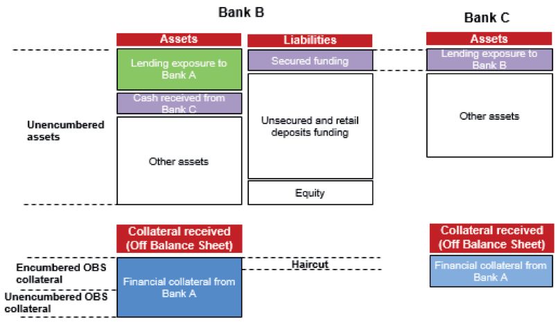
ASSET ENCUMBRANCE AND BANK RISK: THEORY AND FIRST EVIDENCE
FROM PUBLIC DISCLOSURES IN EUROPE
ASSET ENCUMBRANCE AND BANK RISK: THEORY AND FIRST
EVIDENCE FROM PUBLIC DISCLOSURES IN EUROPE (*)

Albert Banal-Estañol
UNIVERSITAT POMPEU FABRA AND BARCELONA GSE

Enrique Benito
CITY, UNIVERSITY OF LONDON

Dmitry Khametshin
BANCO DE ESPAÑA

Jianxing Wei
UNIVERSITY OF INTERNATIONAL BUSINESS AND ECONOMICS

(*) Authors’ contacts: Albert Banal-Estañol, Universitat Pompeu Fabra and Barcelona GSE, albert.banalestanol@
upf.edu; Enrique Benito, City, University of London, enrique.benito.1@city.ac.uk; Dmitry Khametshin, Banco de
España, dmitry.khametshin@bde.es; Jianxing Wei, University of International Business and Economics, jianxing.
wei@uibe.edu.cn. All authors equally contribute to the paper.
Jianxing Wei acknowledges financial support from National Natural Science Foundation of China (Ref. No.
72003030) and University of International Business and Economics (Ref. No. 18QN01). Dmitry Khametshin
acknowledges financial support from the Spanish Ministry of Economy and Competitiveness (BES-2014-070380).
An earlier version of this paper was developed through CEPR’s Restarting European Long-Term Investment
Finance (RELTIF) Programme funded by Emittenti Titoli. We are grateful to Thorsten Beck, Javier Suárez, Florian
Heider, Toni Ahnert, Xavier Freixas, Sergio Mayordomo, Yuliyan Mitkov, Ettore Panetti, Qifei Zhu, José María Liberti,
Andrea Resti, Sergio Schmukler and Mungo Wilson for helpful comments and suggestions, as well as Alexandra
Cahue and Jonas Nieto for excellent research assistance. This work has also benefited from comments by
participants at the 2018 China International Conference in Finance (CICF), Financial Intermediation Research
Society (FIRS) 2019 Conference, ESCB Cluster 3 Financial Stability 2019 Workshop, as well as at the seminars at
Saïd Business School, Cass Business School, Bank of England, Banco de España, and Deutsche Bundesbank.
The views expressed in this paper are those of the authors and should not be attributed to the Banco de España
or the Eurosystem. This draft is from July, 2021.

Documentos de Trabajo. N.º 2131
August 2021
The Working Paper Series seeks to disseminate original research in economics and finance. All papers
have been anonymously refereed. By publishing these papers, the Banco de España aims to contribute
to economic analysis and, in particular, to knowledge of the Spanish economy and its international
environment.

The opinions and analyses in the Working Paper Series are the responsibility of the authors and, therefore,
do not necessarily coincide with those of the Banco de España or the Eurosystem.

The Banco de España disseminates its main reports and most of its publications via the Internet at the
following website: http://www.bde.es.

Reproduction for educational and non-commercial purposes is permitted provided that the source is
acknowledged.

© BANCO DE ESPAÑA, Madrid, 2021

ISSN: 1579-8666 (on line)
Abstract

We document that overcollateralisation of banks’ secured liabilities is positively
associated with the risk premium on their unsecured funding. We rationalize this finding
in a theoretical model in which costs of asset encumbrance increase collateral haircuts
and the endogenous risk of a liquidity-driven bank run. We then test the model’s
predictions using a novel dataset on asset encumbrance of the European banks. Our
empirical analysis demonstrates that banks with more costly asset encumbrance have
higher rates of overcollateralisation and rely less on secured debt. Consistent with theory,
the effects are stronger for banks that are likely to face higher fire-sales discounts. This
evidence acts in favour of the hypothesis that asset encumbrance increases bank risk,
although this relationship is rather heterogeneous.

Keywords: asset encumbrance, collateral, bank risk, credit default swaps.

JEL classification: G01, G21, G28.
Resumen

En este trabajo mostramos que la sobrecolateralización de los pasivos garantizados
bancarios se asocia de forma positiva con la prima de riesgo de su financiación no
garantizada. Incorporamos esta idea en un modelo teórico en el que los costes
derivados del gravamen de activos (asset encumbrance) provocan un aumento de los
descuentos aplicables al colateral (haircuts) y aumentan el riesgo endógeno de una
quiebra bancaria por riesgo de liquidez. Posteriormente comprobamos las predicciones
del modelo utilizando un nuevo conjunto de datos sobre el gravamen de activos de
bancos europeos. El análisis empírico demuestra que los bancos con mayores costes
derivados del gravamen de activos presentan mayores tasas de sobrecolateralización
y menor dependencia de la financiación garantizada. En línea con nuestro modelo
teórico, estos efectos son de mayor magnitud en los bancos que se enfrentan a mayores
descuentos por ventas de activos en situaciones de estrés. Los resultados apuntan
a que el gravamen de activos aumenta el riesgo bancario, aunque esta relación es
bastante heterogénea.

Palabras clave: gravamen de activos, colateral, riesgo bancario, swaps de incumplimiento
crediticio (CDS).

Códigos JEL: G01, G21, G28.
1         Introduction

        Asset encumbrance refers to the existence of bank balance sheet assets being subject to ar-
        rangements that restrict the bank’s ability to transfer or realise them. Assets become encum-
        bered when they are used as collateral to raise (secured) funding, for example in repurchase
        agreements (repos), or in other collateralised transactions such as asset-backed securitisations,
        covered bonds, or derivatives. In stressed situations, high levels of asset encumbrance can im-
        pede obtaining funding and affect the liquidity and solvency of a bank.1 Since bank failures
        can have substantial negative externalities, understanding the effects of asset encumbrance on
        bank default risk is crucial for financial stability.
              Policymakers have acted decisively to address what were considered excessive levels of
        asset encumbrance. Several jurisdictions introduced limits on the level of encumbrance (Aus-
        tralia, New Zealand) or ceilings on the amount of secured funding or covered bonds (Canada,
        US), while others have incorporated encumbrance levels in deposit insurance premiums (Canada).
        Several authors have proposed linking capital requirements to the banks’ asset encumbrance
        levels or establishing further limits to asset encumbrance as a back-stop (Juks (2012), Helberg
        and Lindset (2014), IMF (2013)). As part of the Basel III regulatory package, the Net Stable
        Funding Ratio requires banks to hold higher amounts of stable funding for encumbered assets.
        In Europe, regulatory reporting and disclosure requirements have been introduced and institu-
        tions are required to incorporate asset encumbrance within their risk management frameworks.
        The Dutch National Bank (DNB) even publicly committed to “keeping encumbrance to a min-
        imum” (De Nederlandsche Bank (2016)). This point of view presumes that asset encumbrance
       is detrimental to financial stability. Despite regulatory intervention, the recent outbreak of the
       Covid-19 pandemic has led to a significant increase in asset encumbrance. In Europe, banks
       have made extensive use of new and existing central bank facilities while supervisory con-

            1 InEurope, one can find several examples of bank failures precipitated by high levels of asset encumbrance.
        Dexia, a Franco-Belgian bank that reported a Tier 1 capital ratio of 11.4% and a buffer of e88bn in liquid securi-
        ties as of June 2011, was partly nationalised by the Belgian and French governments in the course of three months
        despite stress tests by the European Banking Authority (EBA) confirming its relatively strong capital position.
        Several commentators highlighted the high levels of encumbered assets as the key factor precipitating its move
        into government arms (e.g., FT (2011)). More than e66bn of Dexia’s e88bn buffer securities were encumbered
        through different secured funding arrangements, particularly with the European Central Bank (ECB), and were
        therefore unavailable for obtaining emergency funding. In June 2017, Spain’s Banco Popular was put into res-
        olution by the European Single Supervisory Mechanism and was acquired by Banco Santander for a symbolic
        amount of e1. Yet, as of year-end 2016, it reported a Tier 1 capital ratio of 12.3% and had passed that year’s EBA
        stress tests with a solid margin. The bank’s disclosures show that nearly 40% of its total balance sheet assets were
        encumbered.

BANCO DE ESPAÑA    7   DOCUMENTO DE TRABAJO N.º 2131
straints on asset encumbrance may have been eased temporarily to support lending.2 In its latest
annual report on Asset Encumbrance, the European Banking Authority (EBA) noted that 2020
registered the largest yearly rise in asset encumbrance since data is available (EBA (2021)).
Asset encumbrance is the product of the level of secured funding chosen by the bank and
its overcollateralisation. In a bank’s private decision, optimising asset encumbrance involves a
trade-off between a bank’s ex-post ability to withstand liquidity shocks and lower ex-ante fund-
ing costs associated with secured finance. Thus, higher levels of asset encumbrance reduce
both the amount of unencumbered assets that the bank can use to meet sudden liquidity de-
mands and the pool of assets that become available to unsecured creditors under insolvency, an
effect coined as structural subordination (see, for instance, CGFS (2013)).3 But by encumber-
ing assets, a bank may also reduce its overall cost of funds and liquidity risks because posting
collateral brings in cheaper and more stable secured funding — this is the stable funding effect
of asset encumbrance. This paper presents a theoretical model exploring this trade-off and pro-
vides empirical evidence on the determinants of asset encumbrance and its relation to the bank
risk premium.
Figure 1 motivates our further analysis. It plots CDS premia on subordinated debt of Eu-
ropean banks in 2015 against overcollateralisation levels of their secured liabilities. On its
vertical axis, the left graph plots banks’ CDS premia on subordinated debt. Similarly, the chart
on the right plots the differential between banks’ CDS premia on subordinated and senior liabil-
ities. On the horizontal axes, we plot overcollateralisation measured as the ratio of encumbered
assets to the matching liabilities using the 2014 asset encumbrance disclosures.4 The figure
illustrates that banks with higher levels of overcollateralisation of their secured liabilities tend
to face higher cost of unsecured funding. The link between the bank risk premium and the
drivers of asset encumbrance is a starting point of our analysis.
[Figure 1]
2 TheDNB, for example, stated: “given the current circumstances, [the] DNB may allow, on a case-by-case
basis, for some temporary relaxation of asset encumbrance limits, provided that this is well substantiated by the
institution concerned” (De Nederlandsche Bank (2020)).
3 As stated by Dr Joachim Nigel, a former member of the Executive Board of the Deutsche Bundesbank, in a
speech at the 2013 European Supervisor Education Conference on the future of European financial supervision:
“Higher asset encumbrance has an impact on unsecured bank creditors. The more bank assets are used for secured
funding, the less remain to secure investors in unsecured instruments in the case of insolvency. They will price in
a risk premium for this form of bank funding”, see Nagel (2013).
4 We provide a detailed description of data construction in Section 3. To ensure that the quality of banks’ assets
and their capital do not drive the relationship in Figure 1, we orthogonalise both the overcollateralisation levels
and CDS premia with respect to banks’ credit ratings and leverage. The regression coefficient (robust standard
error) on overcollateralisation is 4.34 (2.12) for the CDS premium on the subordinated debt, and 1.3 (0.57) for the
excess CDS premium on the subordinated debt net of the senior premium.
BANCO DE ESPAÑA 8 DOCUMENTO DE TRABAJO N.º 2131We rationalize the relationship observed in Figure 1 in a theoretical model in which higher
asset encumbrance costs can increase required overcollateralisation and the endogenous risk
of a liquidity-driven bank run by unsecured investors. In our model, encumbered assets have
higher liquidation costs. These costs may represent value destruction stemming from weaker
monitoring incentives of secured investors or higher price impact in fire-sales of collateral
(Duffie and Skeel (2012)).5 Additionally, encumbrance costs may also include legal costs and
transaction costs of “unencumbering” collateral or transferring assets to the secured creditors in
case of default. The costs of asset encumbrance determine which of its effects — the structural
subordination or stable funding — dominates and, consequently, whether bank risk increases
or decreases with the level of secured financing.
We show that the stable funding effect dominates the adverse impact of structural subordi-
nation when encumbrance costs are relatively low. Indeed, in this case, secured finance reduces
bank risk because, if the bank is to be liquidated, asset encumbrance does not destroy too much
value and leaves plenty of liquidity to the unsecured creditors. On the contrary, when the liq-
uidation costs associated with encumbered assets are high, the amount of liquidity available
after liquidation and paying back the debts to the secured creditors is low. In this case, the
structural subordination effect dominates the one of stable funding, and secured financing in-
creases default risk. Hence, we show that, in theory, the positive relationship between bank
risk and overcollateralisation of secured liabilities is not ubiquitous. Namely, our approach
admits that when costs of asset encumbrance are low, a regulation that limits its levels may be
counterproductive and increase bank risk.
To provide additional insights into which case is empirically relevant, we use the model
to generate further predictions on the relationship between asset encumbrance costs, overcol-
lateralisation, and the optimal choice of secured funding. We show that, in theory, when en-
cumbrance costs are high, they affect the optimal level of secured funding both directly and
indirectly via collateral haircuts.6 Low encumbrance costs, on the contrary, matter for the opti-
mal choice of secured debt only inasmuch as they determine the levels of overcollateralisation.
5 In
our analysis, we do not distinguish between different sources of secured funding but rather analyse the
choice between secured and unsecured finance in general. However, one can extend our framework and incorporate
various modes of securitisation of the same pool of assets characterised by different levels of encumbrance costs.
For instance, a prevalence of asset-backed securitisation over covered bonds issuance in the U.S. can be linked to
higher costs of legal complexity of the latter. From this perspective, one can further relate asset encumbrance to
a more general topic of risk transferring versus risk diversification under different modes of securitisation and its
implications for financial stability. We thank the anonymous referee for pointing this out. While these issues are
of great relevance, we do not address them in this paper since our data does not allow us to differentiate between
various sources of asset encumbrance.
6 Haircut refers to the extent of overcollateralisation. See Gorton and Metrick (2009) and Dang et al. (2013)
for more details.
BANCO DE ESPAÑA 9 DOCUMENTO DE TRABAJO N.º 2131Furthermore, encumbrance, effectively, is more costly when banks losses from a premature
liquidation of their assets are large.
We test these predictions in a cross-section of European banks spanning more than three
hundred institutions from nineteen countries. To do this, we build a novel dataset using the
information provided in the asset encumbrance disclosures published in 2015 by European
banks, following a set of harmonised definitions provided by the EBA (EBA (2014)). We
interpret encumbrance costs from the moral hazard perspective in which secured investors have
weaker incentives to monitor the bank and prevent it from value-destroying activity. From this
perspective, more opaque banks acting in an environment with weaker creditor rights protection
are likely to have higher encumbrance costs. Hence, we use both bank- and country-level
variation and measure encumbrance costs by banks’ opacity and creditors’ rights for filing for
bank bankruptcy.
We show empirically that the encumbrance costs affect the level of secured funding both
directly and via collateral haircuts. Hence, more opaque banks or banks headquartered in coun-
tries that limit creditors’ rights for bankruptcy filing tend to face higher rates of overcollateral-
isation. Accordingly, these banks tend to rely less on secured funding in their capital structure.
Furthermore, encumbrance costs affect the chosen level of secured financing directly, including
when conditioning on collateral haircuts. This evidence acts in favour of the hypothesis that
asset encumbrance increases bank risk. Finally, consistent with the theory, we show that the
direct effect of encumbrance costs is stronger for banks that face potentially higher fire-sales
discounts. This empirical fact implies that the impact of encumbrance costs on bank risk is
rather heterogeneous.
Our paper contributes to a still scarce but growing literature on bank asset encumbrance
and its implications for financial stability. Ahnert et al. (2019) provide a theoretical framework
to study asset encumbrance by banks subject to rollover risk, in which greater encumbrance
allows the bank to attract more funding from secured creditors and increases profitable invest-
ment, but also leads to a higher probability of an unsecured debt run. Our paper also analyzes
asset encumbrance with bank run risk, but differs from Ahnert et al. (2019) in several key re-
spects. First, in our model, banks can use cheap secured finance to replace unsecured funding,
which generates the stable funding effect of asset encumbrance. Thus, we predict that the lev-
els of secured funding can be negatively correlated with the bank risk when encumbrance costs
are low. Second, in our model, encumbrance cost and fire-sales discount jointly determine the
overcollateralisation of secured funding. In Ahnert et al. (2019), on the contrary, overcollat-
BANCO DE ESPAÑA 10 DOCUMENTO DE TRABAJO N.º 2131eralisation is only affected by the recovery rate of encumbered assets upon default. Third, we
provide novel empirical results on the determinants of overcollateralisation and its relation to
bank asset encumbrance and risk, consistent with our theory.7 Our result also differs from Gai
et al. (2013) and Eisenbach et al. (2014) who study the financial stability implications of bank
asset encumbrance in partial equilibrium models with exogenous funding structure.
Empirical analysis of banks’ asset encumbrance is scarce. In the context of interbank mar-
kets, Di Filippo et al. (2016) find that banks with low creditworthiness replace unsecured bor-
rowing with secured loans. Garcia-Appendini et al. (2017) document a positive relationship
between the costs of unsecured debt and asset encumbrance in the context of covered bonds
issuers. Our paper analyses the link between bank risk and asset encumbrance and studies the
determinants of overcollateralisation and secured funding. To the best of our knowledge, our
paper is the first to study this relationship using a broad cross-section of banks not limited to
the largest bond issuers. Finally, we contribute to the literature on law and finance (see, for
instance, Beck, Demirgüç-Kunt, et al. (2003), and Beck and Levine (2008)) by analysing bank
creditor rights protection and financial stability linked by banks’ choice of secured financing.
More generally, our paper is related with the literature on the role of secured debt in cor-
porate financing.8 Our paper is close to Rampini and Viswanathan (2020), who distinguish
between collateral and secured debt and argue that the use of secured debt enables higher lever-
age, but also entails direct and indirect costs. Unlike Rampini and Viswanathan (2020), our
paper focuses on a bank’s funding structure with default risk.
The rest of the paper is organized as follows. Section 2 describes the theoretical framework.
Section 3 provides empirical evidence. In section 4, we discuss the policy implications of our
analysis. Section 5 concludes. Appendix A provides the proofs of the mathematical results,
whereas Appendix B describes the sources of asset encumbrance in the data.
7 Hardy (2014) argues that asset encumbrance reduces liquidation costs and probability of default insofar as
it makes conflict resolution less costly. In our model, this would correspond to low (or negative) encumbrance
costs which would give rise to a negative relationship between secured funding and bank risk. Helberg and
Lindset (2014) study the interplay between asset encumbrance, bank capital, and regulation, and find that “asset
encumbrance increases financial instability from lower optimal capital.” We abstract from the capital and various
regulatory regimes and contribute to their discussion by formulating a simple model in which equilibrium bank
risk can increase due to higher optimal levels of secured funding when the liquidation costs associated with
encumbrance are sufficiently high.
8 In the literature, the possible explanations of the use of secured debt include mitigating agency conflicts
between shareholders and creditors (Smith and Warner (1979), Stulz and Johnson (1985)), addressing the infor-
mation asymmetries between the lender and borrower (Chan and Thakor (1987), Berger and Udell (1990), Thakor
and Udell (1991)), or preventing debt dilution (Donaldson et al. (2020)). See Berger and Udell (1990), Rauh
and Sufi (2010), Luck and Santos (2019), Benmelech et al. (2020) and Lian and Ma (2021) for the empirical
findings on secured debt in corporate financing. A separate line of literature studies the effects of collateral value
and haircuts fluctuations but without referring to the choice of secured vs. unsecured funding. See, for instance,
Brunnermeier and Pedersen (2009) and Adrian and Shin (2010).
BANCO DE ESPAÑA 11 DOCUMENTO DE TRABAJO N.º 21312 Theoretical Framework
We now present a simple model of a bank to understand the decisions about asset encumbrance.
A risk-neutral bank has access to a profitable project that needs one unit of cash at t = 0.
The bank’s project generates a random return θ ≥ 0 at t = 1 and a fixed return k < 1 at t = 2.
The random payoff θ is distributed on the range [0, θ̄ ] with a continuous cumulative distribution
function F with a non-decreasing hazard ratio. As k < 1 and θ can be zero, the bank is subject
to insolvency risk. The bank is protected by limited liability.
At t = 0, the bank has no cash at hand, so it needs to raise funds from a competitive credit
market offering fairly-priced long-term demandable debt. That is, creditors can withdraw their
money at t = 1 before the debt matures at t = 2. To meet creditor withdrawals, the bank can use,
in addition to θ , the proceeds from selling part of the fixed second-period returns k prematurely.
The bank can sell these assets at t = 1 only at a fire-sales discount: the per-unit price at t = 1
is φ < 1.9 The bank fails if the amount of funds withdrawn at t = 1 exceeds its liquid assets.
Thus, the bank is subject to liquidity risk.
The bank raises funding by issuing secured or unsecured debt, so as to maximize the bank’s
expected profits at t = 0. There are two types of creditors. Some are risk-neutral but demand a
minimum expected gross return of 1 + γ, with γ > 0. The others are infinitely risk-averse, and
willing to lend only if debt is absolutely safe, but they demand a minimum return of just 1.10
Since infinitely risk-averse investors demand a lower expected return, it is optimal for the bank
to raise (safe) secured funding from this group of investors, and (risky) unsecured debt from the
risk-neutral investors. This setup captures a major advantage of secure funding: it is perceived
to carry lower roll-over risks and is generally cheaper than equivalent unsecured funding. In
what follows, we refer to γ as risk premium or secured funding gains.
Denote by s the funds raised through secured debt to the risk-averse investors, and by 1 − s
those raised through unsecured debt to the risk-neutral investors. To make sure risk-averse
investors are repaid fully and unconditionally, the bank needs to pledge enough assets. The
bank can use the project’s payoff k at t = 2. The bank’s return θ at t = 1, instead, cannot be
pledged because it is random. Hence, from now on, we refer to k as the available collateral
of the bank, part or all of which can be “encumbered”, i.e., used to raise secured funding.
at t = 1, there is a bond market where the bank can sell, at a price φ , riskless bonds which
9 Equivalently,
promise one unit of cash at t = 2. Since the project’s payoff at t = 2 is k, the bank can sell up to k riskless bonds.
Freixas and Rochet (2008), for instance, use the same setup.
10 A possible interpretation of this assumption is that investors obtain utility directly from holding riskless assets,
see Krishnamurthy and Vissing-Jorgensen (2012), Stein (2012), Caballero and Farhi (2013), W. Diamond (2020)
and Magill et al. (2020) for similar modeling assumptions. Gorton, Lewellen, et al. (2012) and Krishnamurthy
and Vissing-Jorgensen (2012) provide empirical evidence consistent with this assumption.
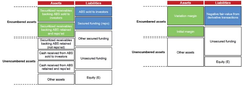
BANCO DE ESPAÑA 12 DOCUMENTO DE TRABAJO N.º 2131This setup captures common sources of asset encumbrance, such as repo financing, securities
financing transactions, or asset-backed securities.11
Encumbering a bank’s assets, however, can be costly. In the model, we capture these fea-
tures through a proportional cost c ≥ 0 associated with secured funding, so that the bank incurs
additional losses cs in case of default.12 We argue that this is a convenient way to capture
multiple sources of costly encumbrance in a simple reduced form.13
The mechanisms generating costs of encumbrance are diverse. For instance, in Calomiris
and Kahn (1991), demandable debt act as an instrument to prevent opportunistic behavior by the
bank managers.14 However, insurance provided by collateral can weaken creditors’ incentives
to monitor the issuer of secured claims. To the extent the lax monitoring by secured investors
can not be easily compensated by other mechanisms, it is likely to exacerbate agency problem
of bank managers and destroy value upon default.
The weaker monitoring pressure by secured investors can manifest itself, among other
things, in stronger incentives of bank managers to postpone filing for bankruptcy. Apart from
direct losses of this gambling for resurrection before resolution takes place, late filings can fur-
ther impact fire-sales prices of the liquidated institution. Duffie and Skeel (2012) discuss these
concerns in more detail. Boyd and Hakenes (2014) and Akerlof et al. (1993) discuss looting
and risk shifting by managers of a bank facing likely default.
Encumbrance costs may also represent legal or transaction costs of transferring assets from
the defaulting bank to the secured creditors (as specified, for instance, in ICMA’s Global Master
Repurchase Agreement). We think, however, that informational frictions described above are
likely to be more important quantitatively.
The resulting maximum amount of secured funding available to the bank at t = 0 is, thus,
φ (1 + c)−1 k. Indeed, for each unit of secured funding, the bank needs to encumber φ −1 (1 +
c) > 1 units of the collateral k, so that the bank can sell it at the fire-sales price at t = 1 and
recover 1 unit, once the encumbrance costs are taken into account. The overcollateralisation or
“haircut”, understood as the difference between the assets’ value and the amount that can be
used as collateral, is thus given by h ≡ 1 − φ (1 + c)−1 . Note that encumbrance costs affect the
11 See Appendix B for further details on sources of asset encumbrance in practice.
12 The assumption that encumbrance costs are incurred by the bank can be generalized to the assumption that
encumbrance is more costly for a defaulting bank than for a surviving one.
13 Similarly, Rampini and Viswanathan (2020) argue that the cost of encumbering assets can either be a direct
cost or an indirect cost due to a loss in operating flexibility, monitoring costs, or the inconvenience of use re-
strictions. Tirole (2006) discusses various costs of pledging assets in corporate finance. See also Jackson and
Kronman (1979), Scott (1996) and Mann (1997) for the discussions of the cost of encumbering asset in the law
literature.
14 See also D. W. Diamond and Rajan (2001).
BANCO DE ESPAÑA 13 DOCUMENTO DE TRABAJO N.º 2131required levels of overcollateralisation since they reduce the amount of resources available to
all creditors upon default.
The encumbered assets cannot be used at t = 1 to meet unsecured debt holders’ withdrawals.
In the event of a “bank run”, secured debt holders can seize the encumbered assets to meet their
claim s. Because of full collateral protection, they have no incentive to withdraw money in the
interim period (i.e., to run the bank). In case of bank failure, the bank distributes any of the
remaining proceeds from selling the long-term assets prematurely φ (1 + c)−1 k − s, along with
θ , on a pro-rata basis to the unsecured investors.
The timing of the model is illustrated in Figure 2.
[Figure 2]
Our model includes several departures from the Modigliani and Miller framework. First, as
it is standard in the banking literature, in the presence of costly asset liquidation, coordination
failure may give rise to bank runs. Furthermore, encumbered assets give rise to additional
liquidation costs, thus reducing the amount of liquidity available to the unsecured investors ex-
post and increasing bank risk and its total debt obligations ex-ante. We turn to the analysis of
the trade-offs of asset encumbrance in the next section.
2.1 Effects of asset encumbrance on bank risk
This section identifies the effects of an exogenous level of secured funding s on the bank’s
risk of failure. Since secured debt is absolutely safe, the face value per unit of secured debt is
equal to 1, which is the minimum return demanded by infinitely risk-averse investors. We first
treat the face value of a unit of unsecured debt, which we denote by D, as exogenously given
and identify the trade-off between structural subordination and stable funding. Thereafter we
endogenise D, taking into account that the risk-neutral investors demand a minimum return of
1 + γ, and identify the key drivers of this trade-off. In the following section, we endogenise the
level of secured funding s and thus the resulting levels of asset encumbrance.
To proceed, we introduce liquidity and solvency thresholds that determine the final out-
come. Thus, the bank is insolvent at t = 1 if and only if the total value of the bank’s assets is
inferior to the total amount of debt obligations, i.e., when θ + k < s(1 + c) + (1 − s)D. Since
k < 1 and θ can be low, there exists a critical solvency return θ such that the bank is insolvent
if and only if θ < θ (s) ≡ s(1 + c) + (1 − s)D − k. In case the realization of θ is low, unse-
BANCO DE ESPAÑA 14 DOCUMENTO DE TRABAJO N.º 2131cured debt holders withdraw their money, thus provoking a (fundamental) bank run. We call θ
solvency threshold.
The bank is not only exposed to insolvency risk but also exposed to liquidity risk. Despite
being solvent, the bank may suffer a bank run at t = 1 if the unsecured investors’ demands
are superior to the bank’s available liquidity. To meet withdrawals, the bank can use its t =
1 proceeds θ as well as proceeds from the fire-sales of long-term assets, net of the amount
recovered by secured creditors, kφ − s, and encumbrance costs, cs. Hence, the bank may suffer
a run if θ + [kφ − s(1 + c)] < (1 − s)D. Rearranging, there exists a critical liquidity threshold
θ , such that the bank is illiquid in case all unsecured investors withdraw if and only if:
θ < θ (s) ≡ (1 − s)D − [kφ − s(1 + c)]. (1)
The range of θ can be split into three regions.15 If θ < θ , the bank is insolvent. If θ <
θ < θ , the bank is solvent but possibly illiquid. If θ > θ , the bank is solvent and liquid. The
intermediate region θ < θ < θ spans multiple equilibria. In one of them, all unsecured debt
holders withdraw and the bank fails. In another equilibrium, all unsecured debt holders choose
not to withdraw and the bank survives. For simplicity, we assume that the bad equilibrium
prevails, so that the bank fails if it is solvent but possibly illiquid, because of the unsecured
investors’ self-fulfilling concern that all the other unsecured debt holders withdraw.16 Since
θ ∼ F(θ ), the bank fails at t = 1 with probability F(θ ) so that bank’s default probability
increases in θ . Given that F is increasing in θ , we call θ a “liquidity threshold” and “bank
default risk” or simply “bank risk” interchangeably.
Notice that an increase in the level of secured funding, s, has two effects on the bank’s
default risk, θ . On the one hand, as s increases (1 − s)D decreases, which implies that the bank
needs less liquidity to face a potential liquidity shock at t = 1. This is the stable funding effect
of secured financing. On the other hand, as s increases, kφ − s(1 + c) decreases, which implies
that the amount of net unencumbered assets available to the unsecured debt holders is lower.
This is the structural subordination effect of secured funding. As we show next, the balance
between the two effects depends on the benefits and costs of using secured funding, γ and c,
respectively.
15 Simplealgebra shows that θ ≤ θ , with the inequality being strict if φ < 1 or c > 0.
16 If
the good equilibrium were to be chosen, bank’s liquidity risk will disappear. In this case, only solvency risk
would be relevant for the bank. Our results would still hold, nevertheless, if we were to allow (more generally) for
an (exogenous) positive probability of failure. In principle, we could also use the global games approach to select
a unique equilibrium (e.g., Rochet and Vives (2004), Goldstein and Pauzner (2005) and Ahnert et al. (2019)). We
work with an exogenously chosen equilibrium for tractability.
BANCO DE ESPAÑA 15 DOCUMENTO DE TRABAJO N.º 2131We endogenise D as following. The face value of the unsecured debt D is determined by
the break-even condition:
θ (s) θ̄
(1 − s)(1 + γ) = (θ + kφ − s(1 + c)) dF + (1 − s)D(s) dF. (2)
0 θ (s)
The first term in the right-hand side is the unsecured debt holders’ expected return in the case of
a bank run: unsecured debt holders share, on a pro-rata basis, the realized return at t = 1, θ , as
well as all the value of the encumbered assets, kφ − s(1 + c). The second term in the right-hand
side is the unsecured debt holder’s expected return when they are fully paid. The left-hand side
is the opportunity cost of the unsecured debt holders’ funding.
Combining (1) and (2), we get the following Proposition:
Proposition 1 If encumbrance costs c are lower (higher) than the risk premium γ, bank risk θ
is decreasing (increasing) in the level of secured funding s.
This result is intuitive. If encumbrance does not impose significant costs on the bank (c < γ),
the amount of liquidity left after recovering the collateral in the case of a bank run is relatively
large. In this case, by exploiting the stability of secured debt, the bank needs less liquidity θ to
meet the withdrawals of the unsecured investors at t = 1: the stable funding effect dominates
the one of structural subordination. If, on the contrary, encumbrance is costly (c > γ), the
amount of liquidity left to the unsecured investors in case of a bank run is small. Hence, for
higher values of secured funding s, the bank is required to have more liquidity θ to compensate
the outflow of unsecured funds at t = 1: the structural subordination effect dominates the one
of stable funding.
2.2 Optimal levels of asset encumbrance
We now examine the bank’s optimal choices of secured funding an asset encumbrance. The
expected profits of the bank at t = 0 are given by:
θ̄
Π= {θ + k − [s + (1 − s)D(s)]} dF (3)
θ (s)
Indeed, when θ < θ , the banks fails due to a bank run at t = 1 and the bank (insiders) get 0.
When θ > θ , the bank survives and the payoff of the bank’s assets is θ + k. At t = 2 the bank
pays s to secured debt holders and (1 − s)D to unsecured investors. Clearly, Π depends on θ
and D, which depend, in turn, on s, as shown in (1) and (2), respectively.
BANCO DE ESPAÑA 16 DOCUMENTO DE TRABAJO N.º 2131Simple algebra shows that, substituting (1) and (2) into (3), we have:
dΠ dF
= γ − cF(θ (s)) − [θ (s) − θ (s) + sc] (θ (s)). (4)
ds ds
The first term shows that a marginal increase in s benefits the bank by allowing it to save γ on
each additional unit of secured funding. The second term states that, for a fixed endogenous
probability of bank failure, the additional unit of secured finance comes at a per-unit cost c
realized upon bank run. The last term describes the effect of encumbrance coming from a
change in the probability of bank run associated with a marginal shift in secured debt. As we
show in the previous section, secured funding can both decrease or increase bank risk, and the
direction of this effect depends on the encumbrance costs c and the funding benefits γ. The
expression in the square brackets, in its turn, can be understood as exposure to this marginal
change in bank risk. It consists of (i) the part of the risky payoff that may be lost due to liquidity
run in excess of the losses coming with the fundamental run, θ − θ , and (ii) direct encumbrance
costs, sc.17 The optimal choice of secured finance, thus, balances its marginal benefits (lower
required return) with marginal costs (additional expected liquidation costs as well as the effects
of encumbrance on the probability of liquidation).
To characterise optimal levels of secured funding further, we consider the two cases: low
and high encumbrance costs relative to the risk premium. When the cost of encumbrance c is
low (c < γ), secured funding affects the bank’s expected profits positively, in two ways. First,
since secured funding is a cheaper source of finance, relative to the costs it has, higher asset
encumbrance reduces bank’s overall funding cost: conditional on success, the bank receives
larger residual payoffs (first two terms in (4)). Second, since c < γ, asset encumbrance reduces
the bank’s liquidity risk (third term in (4)). Thus, the bank sets the level of secured funding as
high as possible.
Proposition 2 If encumbrance costs c are lower than the risk premium γ, the bank’s profits
are strictly increasing in the level of secured funding s, which implies that the optimal level of
secured funding for the bank is s∗ = kφ (1 + c)−1 .
Consider next the case when encumbrance costs are relatively high (c > γ). From Propo-
sition 1 we know that in this case bank’s risk is increasing in the level of secured funding. In
17 Thisterm can equivalently be rewritten as kh − c(k(1 − h) − s). Hence, when the bank uses its full collateral
capacity, s∗ = k(1 − h), the exposure to the marginal change in the bank risk can be measured by the unpledgeable
part of the safe asset, kh. This exposure decreases when the bank chooses a lower level of secured funding.
BANCO DE ESPAÑA 17 DOCUMENTO DE TRABAJO N.º 2131this case the bank may opt not to use its full collateral capacity. In terms of the FOC condition
implied by (4), the bank balances the positive effects of secured funding γ with its unambigu-
ously negative consequences for default risk (a higher expected losses induced by encumbrance
cF(θ ), and a marginal increase in the default probability ds (θ )).
dF
The effect that dominates de-
pends on the level of encumbrance costs c:
Proposition 3 If encumbrance costs c are higher than the risk premium γ, there exist c and c̄,
such that γ < c < c̄ and
(i) bank profits are strictly increasing in the level of secured funding s, so that the optimal
level of secured funding is s∗ = kφ (1 + c)−1 if encumbrance costs are moderately high,
γ < c < c;
(ii) bank profits exhibit an inverted U-shapped form in the level of secured funding s, so that
the optimal level of secured funding is interior, s∗ ∈ (0, kφ (1 + c)−1 ) if encumbrance
costs are significantly high, c < c < c̄;
(iii) bank profits are strictly decreasing in the level of secured funding s, so that the optimal
level of secured funding is s∗ = 0 if encumbrance costs are too high, c > c̄.
Note that when γ < c < c, the bank chooses to use its full collateral capacity, s∗ = k(1 − h).
This equilibrium outcome is identical to the case when c < γ < c. As discussed below, this
result poses challenges for identifying the effect of secured funding on bank risk since the
bank’s optimum alone does not allow to differentiate the two cases.
2.3 Implications for empirical analysis
Propositions 2 and 3 highlight the main conceptual difficulty of empirical identification of the
relationship between bank risk and secured funding. Thus, the propositions suggest that the
bank chooses to use its full collateral capacity whenever encumbrance costs are relatively low,
i.e., when c < c. However, as suggested by the Proposition 1, this fact alone does not identify
the dependence of bank risk on secured funding as the latter may have positive or negative
effect on bank risk whenever γ < c < c or c < γ < c, correspondingly. Similarly, one can show
that, in equilibrium, the price of unsecured debt, D, is positively related to encumbrance costs
c whenever c < c. In this case, the bank uses its full collateral capacity, s∗ = k(1 − h), and
θ (k(1−h))
the cost of the unsecured debt is D∗ = 1−k(1−h) . Taking into account that dθ
dh > 0 and dh
dc > 0,
BANCO DE ESPAÑA 18 DOCUMENTO DE TRABAJO N.º 2131dD∗
we have dc > 0.18 It follows, that the positive relationship between the cost of the unsecured
debt, D, and the level of overcollateralisation, h, can be obtained both when encumbrance costs
are low, c < γ < c, or moderately high, γ < c < c. Hence, in our model, observing high levels
of secured funding or its positive correlation with the cost of unsecured debt do not necessarily
imply that, if the bank was constrained to reduce its encumbrance ratio, the default risk would
have gone down.
Still, Proposition 3 suggests a way to differentiate between moderately high and signifi-
cantly high encumbrance costs. This comparison, in its turn, is informative about the sign of
the sensitivity of bank risk with respect to secured funding. We formulate this result as the
following corollary.
Corollary 1 An increase in encumbrance costs c when haircut h is held fixed (i) does not affect
the optimal level of secured funding s∗ if c < c, and (ii) decreases the optimal level of secured
funding s∗ if c < c < c̄.
In the model, encumbrance costs affect the haircut on secured funding because they reduce the
amount of liquidity available to all creditors upon default. Hence, collateralisability of the safe
asset decreases as encumbrance costs increase. If these costs are relatively low (c < c), the bank
chooses maximum available secured funding, s∗ = k(1 − h(c, φ )): in this case, encumbrance
costs propagate to the choice of funding structure only via collateral haircut.
Corollary 1 highlights that, apart from affecting the choice of secured funding via haircut,
asset encumbrance has another — direct — effect on the optimal funding structure. This effect
manifests itself in the bank’s optimal decision whenever encumbrance costs are sufficiently
high (c < c < c̄). In this case, the bank chooses to operate at the interior optimum below its full
collateral capacity, s∗ < k(1 − h), to reduce marginal costs of secured debt. As discussed above,
lowering these costs involves reducing expected per-unit losses from encumbrance, decreasing
the sensitivity of default probability to the choice of s, and lowering the bank’s exposure to the
changes in default probability. All three components of marginal costs depend positively on
encumbrance costs, even when the collateral haircut is held fixed. In the interior optimum, this
results in a negative dependence of secured funding on the costs of asset encumbrance — in
addition to the effects of the latter mediated via haircut.
Corollary 1, when coupled with the Proposition 1, shows that the presence of the direct neg-
ative effect of encumbrance costs on the level secured funding is indicative of unambiguously
results holds whenever (1 + γ)(1 − k(1 − h)) > θ (k(1 − h))(1 − F(θ (k(1 − h)))) which holds from the
18 This
break-even condition.
BANCO DE ESPAÑA 19 DOCUMENTO DE TRABAJO N.º 2131positive relationship between the latter and bank risk. We use this model conclusion extensively
as a guidance for the empirical analysis below.
Another implication for the interpretation of empirical evidence concerns the role of fire-
sales prices. Intuitively, fire-sales price determines the minimum losses of a bank’s liquidity
that do not depend on its funding structure. Hence, with high fire-sales discounts, even small
encumbrance costs can hurt the bank by further draining its liquidity ex-post and increasing
the probability of bank run ex-ante. In other words, the bank can perceive the same level of
encumbrance costs as low when it does not lose too much value in fire-sales and high — if asset
liquidation is exceptionally costly. We formalize this intuition in the following corollary.
Corollary 2 The encumbrance cost threshold c, that separates interior optimum from the case
of full collateral utilisation, is high when fire-sales discount is low:
dc
> 0.
dφ
Corollary 2 suggests that conditional on the level of overcollateralisation, encumbrance
costs are more likely to directly affect the chosen level of secured funding when fire-sales dis-
counts are high. We use this conclusion in the next section, where we analyse the dependence
of secured funding on encumbrance costs empirically.
3 Empirical evidence
Figure 1 that motivated our analysis so far is indicative of a positive relationship between se-
cured funding and bank risk. Yet, as discussed above, this fact alone may not be sufficient to
conclude that secured finance increases bank risk. In this section, we provide further empiri-
cal evidence on the relationship between encumbrance costs, overcollateralisation, and secured
funding using a larger cross-section of European banks. Our general empirical strategy is as fol-
lows. We first analyse the determinants of overcollateralisation across banks. Having identified
the variables that are likely to be related to the theoretical concept of costs of asset encum-
brance, we move on to the analysis of the determinants of bank’s reliance on secured funding.
Following our theoretical results, we are mostly interested in the drivers of secured funding
conditional on the haircuts faced by the banks. In particular, to interpret the empirical observa-
tions, we employ Corollary 1 and analyse whether proxies of encumbrance costs correlate with
the choice of secured funding beyond the effects of the former on overcollateralisation. Finally,
BANCO DE ESPAÑA 20 DOCUMENTO DE TRABAJO N.º 2131guided by Corollary 2, we analyse the heterogeneity of the relationship between encumbrance
costs and secured finance in its relation to the potential magnitude of fire-sales discounts.
3.1 Data and Descriptive Statistics
Asset encumbrance, balance sheet, and macroeconomic data. Computing asset encumbrance
measures at the bank level is not straightforward since standard accounting data provides lim-
ited information to infer the amount of banks’ encumbered assets, unencumbered assets and
matching liabilities. Accounting statements are accompanied by disclosures which try to shed
light on the amount of assets that collateralise transactions but, as noted by the EBA: “existing
disclosures in International Financial Reporting Standards may convey certain situations of en-
cumbrance but fail to provide a comprehensive view on the phenomenon” (EBA (2014)). For
this reason, the EBA introduced new guidelines in 2014 proposing the requirement to disclose
asset encumbrance reporting templates. EBA guidelines do not constitute a regulatory require-
ment and, although most did, not all of the European institutions disclosed such information.
We start the empirical analysis by selecting the sample of EU banks whose total assets
exceed e 1 mn. as of the end of 2014. For each bank, we collect risk disclosures from its web
page and extract the reported encumbrance data from the reporting templates suggested by
the EBA. The data includes information on encumbered and unencumbered assets, off-balance
sheet (OBS) collateral received and available for encumbrance, OBS collateral received and re-
used, and matching liabilities (the liabilities or obligations that give rise to encumbered assets).
The encumbrance data we use in this paper is as of year-end 2014. Our main sample includes
306 banks from 19 countries.19
To calculate bank-level values of secured funding and corresponding collateral haircuts, we
rely on the reported values of total encumbered assets, total unencumbered assets, and matching
liabilities. We include encumbered off-balance positions of the bank in calculating haircuts.
Reporting of matching liabilities is of somewhat lower quality than the one of encumbered
assets. Hence, about 14% of banks that disclose asset encumbrance do not disclose the value
of matching liabilities. These banks are mostly small local lenders, and we do not include them
in our final sample.
We calculate the haircut on bank secured lending as the difference between the total value
of encumbered assets and matching liabilities divided by the former. Furthermore, we calculate
19 Countries
included in the sample are Austria, Belgium, Bulgaria, Cyprus, Germany, Denmark, Spain, France,
the United Kingdom, Greece, Croatia, Hungary, Ireland, Italy, Luxembourg, the Netherlands, Portugal, Sweden,
and Slovenia.
BANCO DE ESPAÑA 21 DOCUMENTO DE TRABAJO N.º 2131secured funding as the ratio of matching liabilities to the sum of encumbered and unencumbered
assets. With these definitions, both variables are constructed using information solely from the
disclosed risk reports. As an alternative definition and robustness check we use the ratio of
matching liabilities to total liabilities as a measure of secured funding, where the liabilities are
incurred from the Bankscope database. We get results similar to the ones reported below when
using this auxiliary definition of total liabilities.
We complement this information with bank balance sheet data from Bankscope to capture
known determinants of bank risk. The control variables include proxies for bank profitability
(ratio of net interest revenue to total assets), quality of credit portfolio (share of non-performing
loans in total loans), leverage (ratio of common equity to total assets), liquidity (deposits and
short-term funding, and liquid assets, both normalized by total assets), and bank size (measured
by the natural logarithm of total assets).20 Furthermore, we include a dummy variable to iden-
tify which banks are of investment grade. We use implied ratings provided by Fitch Solutions
and derived from proprietary fundamental data. These provide a forward-looking assessment
of the stand-alone financial strength of a bank and are categorized according to a 10-point rat-
ing. Finally, we include dummy variables to differentiate the business model of the institution
using four categories: “Commercial banks and Bank holding companies (BHC)”, “cooperative
banks”, “savings banks”, “real estate banks”, and “other banks.”
To account for potential sources of omitted variable bias at the country level, we expand
the list of control variables to include macroeconomic indicators. In particular, we use net
foreign assets of depository institutions normalized by a country’s GDP to capture banking
sector reliance on foreign funding (we obtain the data from International Financial Statistics of
IMF). We also control for the marketability structure of financial system liabilities measured
by the difference between security and loan liabilities of a country’s financial corporations
normalized by GDP (the data is obtained from Financial balance sheets of Eurostat). To capture
the differences in deposit insurance systems across the countries, we use the Deposit Guarantee
Scheme (DGS) Moral Hazard index from Demirgüç-Kunt et al. (2014). The latter aggregates
multiple characteristics of a country’s safety net in a way that higher values stand for “more
generosity or greater government support and imply more moral hazard.”21 Finally, we add a
dummy variable for banks headquartered in Greece, Ireland, Italy, Portugal, and Spain (GIIPS)
20 Somesources of asset encumbrance, such as securitisation, involve substantial costs of a fixed nature, which
may be particularly relevant for smaller banks (Adrian and Shin (2010), Carbó-Valverde et al. (2012), Panetta and
Pozzolo (2018)).
21 Ahnert et al. (2019) predict that banks have incentives to increase asset encumbrance to take advantage of
deposit insurance.
BANCO DE ESPAÑA 22 DOCUMENTO DE TRABAJO N.º 2131dummy variable for banks headquartered in Greece, Ireland, Italy, Portugal, and Spain (GIIPS)
and the Eurozone indicator to account for the heterogeneity of banks within the Euro Area and,
more generally, within the EU.
Costs of asset encumbrance. Measuring potential encumbrance costs is notoriously difficult.
Since no directly observable measures are available, we opt for using variables that are likely to
serve as proxies for encumbrance costs from the perspective of the economic model described
above. In particular, as described in the previous section, insolvency costs specific to secured
financing can be related to agency problems that arise due to weaker monitoring incentives of
the secured investors. Hence, we assume that encumbrance costs are higher for banks that are
more difficult to monitor and use bank- and country-level variables that are likely to capture
these agency frictions.
At the country level, we explore variation in bank resolution frameworks of the European
countries. To do this, we rely on a “Study on the differences between bank insolvency laws and
on their potential harmonisation” by the European Commission (Buckingham et al. (2019)).
The Study analyses differences in the legislative regimes applicable at the national level to
bank insolvency proceedings. It provides a qualitative description of resolution mechanisms in
the EU member states along several dimensions, including differences in objectives of insol-
vency procedures, pre-insolvency activity, definitions of bank insolvency, and administrative
proceedings in bank liquidation and administration.22 We use the Study’s section on “Standing
to file insolvency” to identify member states that allow creditors to initiate insolvency proceed-
ings. While in most of the countries of the EU the process can be commenced by the national
competent authority, only half of the member states grant similar rights to creditors. Hence, we
construct an indicator variable “Insolvency filing by creditor” equal to one for banks that are
headquartered in countries where bank creditors can initiate insolvency proceedings, and zero
otherwise.23 We maintain that the right of the unsecured creditors to file for bankruptcy can
serve as a threat to the bank managers preventing them from engaging in a value-destroying
activity. To the extent this creditors’ right of filing for insolvency can partially compensate for
22 Thelegislative regimes applicable at a national level to bank insolvency proceedings can be very different
from the ones applied to corporate insolvency in general. Buckingham et al. (2019) provide further details on
this point. This difference in provisions governing bank insolvency and general corporate insolvency is the main
reason why we opt for using the Commission’s report as our source of creditors’ protection classification. Also,
since the report focuses on the EU, it covers all its member states in great detail, which may not be the case with
other sources, such as the World Bank Doing Business database.
23 The EU Member States that allow creditors to initiate insolvency proceedings are Belgium, Cyprus, Czech
Republic, Denmark, Estonia, Spain, Finland, France, Latvia, Lithuania, Malta, Romania, and Sweden.
BANCO DE ESPAÑA 23 DOCUMENTO DE TRABAJO N.º 2131You can also read