2021 Summer Course on Optical Oceanography and Ocean Color Remote Sensing Monte Carlo Simulation - Curtis Mobley - Maine In-situ Sound & Color Lab

2021 Summer Course
on Optical Oceanography and
Ocean Color Remote Sensing

         Curtis Mobley

  Monte Carlo Simulation

     Schiller Coastal Studies Center

        Copyright © 2021 by Curtis D. Mobley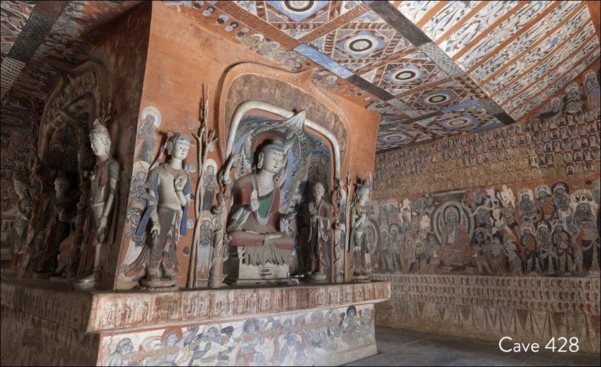

Hey Curt,
  wanna go to
 my place and,
 uh, talk about
    radiative
transfer theory?   Not tonight.
                     I’m still
                   debugging
                   my new 3D
                   Monte Carlo
                       code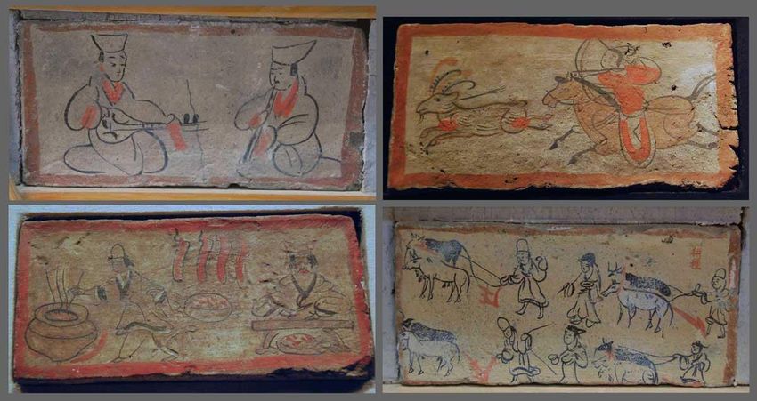

Example 3D Radiative Transfer Problems
           (which can’t be solved by the 1D HydroLight)

                 sloping or patchy bottoms

Mobley and Sundman, 2002                 Mobley, 2018; Lesser et al., 2021

Example 3D Radiative Transfer Problems
          (which can’t be solved by the 1D HydroLight)

objects in the water, or instrument and ship shadow effects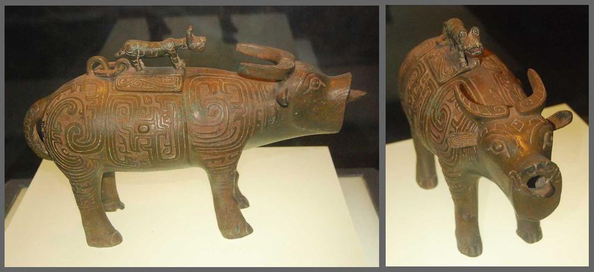

Monte Carlo Techniques
Monte Carlo techniques refer to the use of probability theory and
random numbers to simulate a physical process.

An essential feature of Monte Carlo simulation is that the known
probability of occurrence of each separate event in a sequence
of events is used to estimate the probability of the occurrence
of the entire sequence.

In the optics setting, the known probabilities that a light ray (often
called a “photon packet”) will travel a certain distance, be scattered
through a certain angle, reflect off a surface in a certain direction,
etc., are used to estimate the probability that a ray emitted from a
source at one location will travel through the medium and eventually
be recorded by a detector at a different location.

Averages over ensembles of large numbers of simulated ray
trajectories give statistical estimates of radiances, irradiances,
and other quantities of interest.

Monte Carlo Techniques for Solving the RTE
 The basic idea:

• Mimic nature in the generation and propagation of light rays

• Build up a solution to the RTE one ray at a time

• The tools for doing this are basic probability theory and a random
number generator

Monte Carlo Techniques for Solving the RTE

  Topics to be covered:

• Probability distribution functions (PDFs) and cumulative distribution
functions (CDFs)

• Random number generators

• Using CDFs to randomly select distances, scattering angles, etc.

• Monte Carlo noise

There are web book pages on Monte Carlo techniques starting at
https://www.oceanopticsbook.info/view/monte-carlo-simulation/introduction
and see Chapter 12 of the OOB.

Probability Density Functions

A probability density function (PDF) is a non-negative function p(x) such that
the probability that its variable x is between x and x+dx is p(x)dx.

Example: x = height of adult humans

                                           Probability that a person selected
                                           at random from all humans is
p(x) [1/m]

                                           between 1.0 and 1.3 m tall is

             0   1           2   3
                     x [m]

   Normalization:                    that is, the prob is one that a person

   will have some height between 0 and ∞

   Units of p(x) are always 1/[x]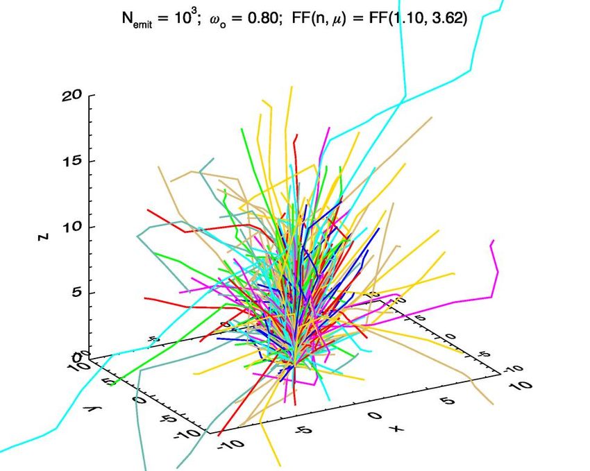

Cumulative Distribution Functions
A cumulative distribution function (CDF) is a non-negative function CDF(x)
such that the probability that its variable has a value ≤ x is CDF(x). For the
human height example,

                                          Probability that a person selected
     1                                    at random from all humans is
                                          between 1.0 and 1.3 m tall is
CDF(x)

                                          CDF(1.3) – CDF(1.0)

     0
         0   1           2   3
                 x [m]

 Note that CDF(∞) = 1. That is, the probability is one that a person will
 have some height less than ∞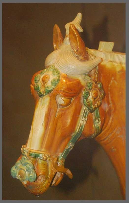

U(0,1) Random Number Generators

                                        p(R)
A Uniform 0-1 random number
generator is anything (usually a
computer program) that when called       1
returns a number R between 0 and
1 with equal probability of returning
any value 0 < R < 1. R ~ U(0,1)           0
                                               0     1          R

       0.6314325330
       0.2641695440
       0.7653187510
       0.3009850980
       0.9278188350
       0.0138932914
       0.3010187450
       0.1198131440                       100 bins, 0.01 wide
       0.3243462440
       0.3493790630
       0.1154079510
       0.1382016390
       0.1065650730

Which Sequence of Numbers is Probably NOT Random?

  452878231035972340523765091082725314057609439765120372140674….

  142983211983496178801321756333339673012007362876201847772190….

Which Arrangement of Dots is Probably NOT Random?

Light Rays
A light ray is a hypothetical construct that indicates the direction of
the propagation of light at any point in space.

This idea is based on the every-day observation that light travels in
straight lines (in a homogeneous medium).

Geometric optics is an approximate
model of light propagation that holds
when the scattering particles (or
lenses, mirrors, etc.) are much, much
larger than the wavelength, so that
diffraction and interference can be
ignored. Light rays are the basic
“objects” of geometrical optics.
Geometric optics and very
sophisticated ray tracing programs
are used to design camera lenses.

Random Determination of Ray Path Lengths
Recall Beer’s law (for a collimated beam in a dark, homogeneous ocean):

The exponential decay of radiance can be explained if the individual rays
have a probability of being absorbed or scattered out of the beam between τ
and τ+dτ that is

We want to use our U(0,1) random number generator to randomly determine
ray path lengths τ that obey the pdf p(τ) = exp(-τ). Going from R to τ is a
change of variables:

Random Determination of Ray Path Lengths

Solving

gives

Draw a U[0,1] random number R, and then the
corresponding ray path length is

or

            for distances r in meters.

Fundamental Principle of MC Simulation

The equation R = CDF(x)                       1

                                     CDF(x)
uniquely determines x                         R
such that x obeys the
corresponding pdf p(x)
                                              0
                                                     x           x

General procedure:

1.   Figure out the pdf p(x) that governs the variable of interest, x
2.   Compute the corresponding CDF(x)
3.   Draw a U[0,1] random number R
4.   Solve R = CDF(x) for x
5.   Repeat steps 3 and 4 many, many, many times to generate a
     sample of x values that reproduces the behavior of x in nature

Mean Free Path
The pdf for the distance a ray travels is p(τ) = exp(-τ).
What is the average distance  that a ray travels?
Called the mean free path.

or, since τ = cr,

 = 1/c (meters)

What is the variance about the mean distance traveled?

so the standard deviation is also 1/c (meters)

Random Determination of Scattering Angles

                   Scattering is inherently 3D:

                   ψ is polar scattering angle

                   χ is azimuthal scattering angle

                                phase functions can be
                                interpreted as pdfs for
                                scattering from (ψ′, χ′)
                                to (ψ, χ)

Random Determination of Scattering Angles
For isotropic media and unpolarzed light, ψ and χ are independent,
so the bivariate pdf is the product of 2 pdfs:

Any azimuthal angle 0 ≤ χ < 2π is equally likely:

                                                    solve for ψ
                                                    (usually must solve
                                                    numerically)

Example: Isotropic Scattering

Example: Isotropic Scattering
  For isotropic scattering,

                          gives

Isotropic means equally likely to scatter into any element of solid angle, not
equally likely to scatter through any polar scattering angle ψ

Tracing Rays
The albedo of single scattering, ωo = b/c, is the probability that a ray (or
photon) will be scattered, rather than absorbed, in any interaction

What nature does:
• draws a random number and gets the distance
• draws another random number and compares with ωo :
   ▪ if R > ωo the ray (photon) is absorbed; start another one
   ▪ if R ≤ ωo the ray (photon) is scattered; compute the scattering
      angles

Any ray that is absorbed never contributes to the answer and is wasted
computation. Nature can afford to waste rays; scientists cannot.

Tracing Ray Bundles
Rather that lose some rays to absorption, consider each ray to be a
bundle of many parallel rays starting with power w = 1 Watt. At each
interaction, multiply the current weight w by ωo to account for loss of
some of the original power to absorption. This increases the number
of rays that contribute to the answer (although some may still miss the
target).

Usually kill the ray when w < 10-8, for example, if it hasn’t hit the
target.

Visualizing
Ray Paths

Visualizing Ray Paths
             Monte Carlo simulation gives
             understanding at the individual
             ray level, which can’t be
             obtained from radiance (e.g.,
             from HydroLight)

30 deg
off axis

Statistical Noise
   The answer you get depends on random numbers and on the number
   of rays collected, so it has statistical noise, aka Monte Carlo noise.

                                                        Repeated runs
                                                        (different sequences
                                                        of random numbers)
                                                        with the same
                                                        number of rays per
                                                        run.

                                                        Note that as more
                                                        runs are done, the
distribution of errors in the estimated mean            distribution of
                                                        computed values
                                                        (errors) approaches
                                                        a Gaussian:

                                                        The Central Limit
                                                        Theorem in action

Statistical Noise
Is the spread of the estimates (coefficient of variance) too large?
Trace more rays...
                                                       The same numbers
                                                       of runs , but with
                                                       more rays per run.

                                                       The variance in the
                                                       computed values is
                                                       ~1/N, N = number
                                                       of rays detected

                                                        To reduce the std
                                                        dev of the
                                                        estimate by a
                                                        factor of 10, must
                                                        detect 100 times
                                                        more rays

Variance Reduction
You now know enough to do the Monte Carlo lab.

However, before writing your own MC code to do extensive
simulations, read about other ways to get more rays onto the target
without more computer time (see the Web Book Monte Carlo chapter).
These are generally called “variance reduction” techniques, and there
are many (“backward ray tracing”, “importance sampling,”, “forced
collisions”,...)

In general:

• First, figure out how to simulate what nature does

• Then figure out how to redo the calculations to maximize the
  number of rays detected (i.e., solve a different problem that has the
  same answer as the original problem—variance reduction)

• The goal (seldom attained) is to Never Waste a Ray

Variance Reduction: Backward Monte Carlo
Emit rays from the detector with weight w = 1 and the angular distribution of
the detector response, and trace to the source. Then weight the “detected”
rays at the source to apply the correct source weight. Only ray paths
conecting the true source (e.g., the sky) and the true detector are then traced.

                                                    The Principle of
                                                    Electromagnetic
                                                    Reciprocity says that a ray
                                                    will trace the same path
                                                    going in either direction
                                                    (If I can see you, you can
                                                    see me.)

                                                Mobley and Sundman, L&O, 2003

Variance Reduction: Backward Monte Carlo
                                     After ray tracing (with
Each sky quad
                                     rays from the detector to
records the fraction of
                                     the sky) is complete,
power emitted from
                                     then apply a sky
the detector that
                                     radiance model to
reaches the quad.
                                     compute the total power
                                     from the sky that would
                                     reach the Ed detector
                                     (with the rays going from
                                     sky to detector)

   Forward MC: an Ed                Backward MC: an Ed
   detector has a cosine            detector has a cosine
   response                         emission pattern

Example: Backward Monte Carlo
Developing a shadow correction for the Lee method.

                                 (from Shang et al, 2017)

Example: Backward Monte Carlo

First they compared their BMC code with HydroLight, for no
instrument present (1 D geometry); agreement to within 1%

Then they compared their
BMC results with Gordon
and Ding (1992) for the
geometry of GD92
(cylindrical instrument, didn’t
study backscatter effects)

Then they did simulations on
a super computer for their
instrument geometry and
developed a shading
correction for their specific
instrument as a function of
a, bb, sun zenith angle.

Monte Carlo Strengths
▪ They are conceptually simple. The methods are based on a
  straightforward mimicry of nature.

▪ They are very general. Monte Carlo simulations can be used to
  solve problems for any geometry (e.g., 3D volumes with imbedded
  objects), incident lighting, scattering phase functions, etc. It is
  relatively easy to include polarization and time dependence.

▪ They are instructive. The solution algorithms highlight the
  fundamental processes of absorption and scattering, and they
  make clear the connections between the ray-level and the energy-
  level formulations of radiative transfer theory.

▪ They are relatively simple to program. The resulting computer
  code can be simple (compared to other techniques), and the
  tracing of rays is well suited to parallel processing.

Monte Carlo Weaknesses

▪ They can be computationally very inefficient. Monte Carlo
  simulation is inherently a “brute force” technique. If care is not
  taken, much of the computational time can be expended tracing
  rays that never contribute to the solution, e.g., because they
  never intercept a simulated detector.

▪ They are not well suited for some types of problems. For
  example, computations of radiance at large optical depths can
  require unacceptably large amounts of computer time because
  the number of solar rays penetrating the ocean decreases
  exponentially with the optical depth. Likewise, the simulation of
  a small source and a small detector is difficult.

▪ They provide no insight into the underlying mathematical
  structure of radiative transfer theory. The simulations simply
  accumulate the results of tracing large numbers of rays, each of
  which is independent of the others.

Following Marco Polo Along the Silk Road in Western China

Tang tri-color horse and camel
Shaanxi Provincial Museum, Xi’an; Tang 618–907)

Bronze wine jug, Western Zhou Dynasty (1000-900 BC),
          Shaanxi Provincial Museum, Xi’an

Tomb bricks, Gobi Desert near Jiayuguan, Gansu Province. Wei-Jin era (200-400 AD)

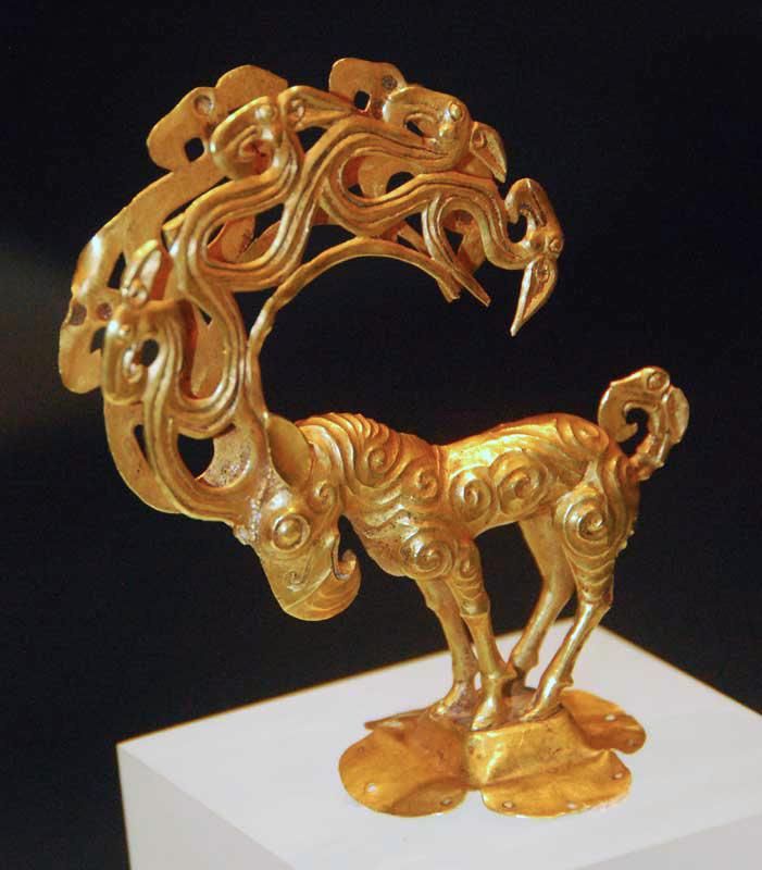
Gold ibex (?) and Teapot, Shaanxi Provincial Museum, Xi’an

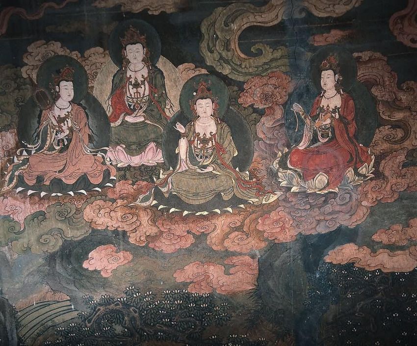
Mogau Grottos near Dunhuang (c 400 – 1500 AD)

                      http://www.xrez.com/blog/mogao-caves-vr/

https://www.askideas.com/30-most-beautiful-paintings-inside-the-mogao-caves-in-dunhuang-china/

The Flying Horse of Gansu, Han (25-200 CE)
    Gansu Provincial Museum, Lanzhou