A Cooperative Game Theory Application and Economical Behavior in an Aspect of Bangladesh with a Real- Life Problem - IOSR Journal

IOSR Journal of Mathematics (IOSR-JM)
e-ISSN: 2278-5728, p-ISSN: 2319-765X. Volume 16, Issue 3 Ser. III (May – June 2020), PP 06-10
www.iosrjournals.org

 A Cooperative Game Theory Application and Economical
 Behavior in an Aspect of Bangladesh with a Real- Life Problem.
 Md Obaidul Haque1, Zillur Rahman2, Sharmin Akter3
 1
 (Department of Mathematics, Comilla University, Bangladesh)
 2
 (Assistant Professor, Department of Mathematics, Comilla University, Bangladesh)
 3
 (Department of Mathematics, Comilla University, Bangladesh)

Abstract: Cooperative game theory made a great impression on several aspects of life sciences and the
impression of scientific theory had started fifty years ago. This research paper illustrates a top-level view of the
implementation of skills gained by students in Mathematics for Business and Economics to unravel problems of
the game theory. Economically speaking, people have choices, demands, wishes, and desires. While it's expected
that individuals will act in a very rational way to comply with social norms, the method is complicated thanks to
external factors like prices, production, gains, and expenses. The act of constructing a rational decision
regarding choices involves what's said as a social exchange economy.
Key Word: Game Theory, Cooperative Game, Strategy, Player, Zero Sum Game, Penalty, Equilibrium, Payoff
Matrix, Probability.
---------------------------------------------------------------------------------------------------------------------------------------
Date of Submission: 13-05-2020 Date of Acceptance: 25-05-2020
---------------------------------------------------------------------------------------------------------------------------------------

 I. Introduction
 Game theory is an autonomous discipline that is used in applied mathematics, social sciences, most
remarkably in mathematics, economics, as well as in computer science, biology, engineering, international
relations, philosophy, and political science. It was displayed in economics and mathematics to measure
economic behaviors including behaviors of firms, markets, and consumers. The cooperative game theory can be
contemplated as a modeling procedure that is used to analyze and explain the actions of all players joined in
competitive situations and to compare and determine the relative optimality of distinct strategies. The first
inspect of games in terms of economics was by Cournot in 1838 on pricing and production but John von
Neumann is considered as the founder of the modem game theory. In cooperative game theory, it can be said
that the set of bounded computational capacity of equilibrium payoffs carries only one valuation, that the
valuation of the game with penalty approaches the valuation of the one-shot game as the penalty goes to zero.
The goal is to anticipate moves to ready, which is able to cause ultimate victory.

 II. Mathematical Formulation
Let us consider two players’ and (two-person zero-sum game). Each chooses one of the possible strategies
 ( = 1, ) and ( = 1, ).
Let 1 ( ; )( = 1, ; = 1, ) when Player wins; and 2 ( ; )( = 1, ; = 1, ) when Player 
wins.
Since we have a zero-sum game, 1 ( ; )+ 2 ( ; )= 0.
We have 1 ( ; ) = ( ; ) and 2 ( ; )= − ( ; )
Thus, the goal of Player is to maximize the value ( ; )and Player minimize it. Suppose that
 ( ; ) = , we have the matrix :
 11 12 … … … 1 
 21 22 … … … 2 
 X =( … … … … … … … … … ) … … … … … (1)
 1 2 … … … 
where rows correspond to the strategies and columns to the strategies . The matrix is called the payoff
matrix. An element of this matrix is when Player wins if he/she had chosen strategy, and Player had
chosen the strategy. Player has to choose the strategy to maximize his/her minimum payoffs, such as:
 = 
 
 … … … … … … … … (2)
The amount of the loss is called the upper value of the game:
 = 
 
 … … … … … … … ... (3)

DOI: 10.9790/5728-1603030610 www.iosrjournals.org 6 | Page

A Cooperative Game Theory Application and Economical Behavior in an Aspect of Bangladesh …

If 
 
 = 
 
 = , the game is called well-defined. But if ≠ , ≤ ≤ , its maximin –
minimax strategies are not optimal. This means that each party can improve its results by choosing a different
approach. The optimal solution for such a game is mixed strategies, which are the specific combinations of the
original “pure” strategies.
For Player vector = ( 1 , 2 , 3 , … … … , ) , where ∑ =1 = 1
For Player vector = ( 1 , 2 , 3 , … … … , ) , where ∑ =1 = 1
 ≥ 0( = 1, ); ≥ 0 ( = 1, )
It appears that when the mixed strategies are used, for every finite game one can find a couple of stable optimal
strategies. The main theorem of game theory determines the existence of a solution. The main theorem of game
theory says that every finite game has at least one solution which is possible in mixed strategies.
Suppose we have a finite matrix game with the payoff matrix (1). According to the theorem, optimal mixed
strategies for players are determined by vectors
 ∗ = ( 1 ∗ , 2 ∗ , 3 ∗ , … … , ∗ ) and ∗ = ( 1 ∗ , 2 ∗ , 3 ∗ , … … , ∗), which give the possibility to receive the win:
 ≤ ≤ .
Using the optimal mixed strategy should provide Player with a certain payoff that is not less than the value of
the game. Mathematically, this condition is written as:
 ∑ ∗
 =1 ≥ ( = 1, ) … … … … ... (4)
On the other hand, the use of an optimal mixed strategy for Player should provide, for any strategy that Player
 chooses, the loss that is not exceeding the value of the game, that is:
 ∑ ∗
 =1 ≤ ( = 1, ) … … … … … … (5)
These relationships are used to find the solution of the game. We need to find the mixed strategies and the value
of the game. Denote the desired probabilities value for the Player in the “pure” strategies with ∗ = ( 1 ∗ , 2 ∗ )
and for player with ∗ = ( 1 ∗ , 2 ∗ ) .
According to the main game theory theorem, if the player sticks to its optimal strategy, the payoff will be equal
to the value of the game.
So if Player sticks to his/her optimal strategy ∗ = ( 1 ∗ , 2 ∗ ), then:
 ∗ + 21 2 ∗ = 
 { 11 1 ∗ … … … … … … (6)
 12 1 + 22 2 ∗ = 
Since 1 ∗ + 2 ∗ = 1, then 2 ∗ = 1 − 1 ∗ . Substituting this expression into the system (6), we obtain:
 ∗ + 21 (1 − 1 ∗ ) = 
 { 11 1 ∗
 12 1 + 22 (1 − 1 ∗ ) = 
 Or, 11 1 ∗ + 21 (1 − 1 ∗ ) = 12 1 ∗ + 22 (1 − 1 ∗ )
Solving this equation, we have,
 21
 1 ∗ = + 22− … … … … … ... (7)
 11 22 − − 
 12 21
And,
 22− 21 11− 12
 2 ∗ = 1 − 1 ∗ = 1 − = … … … … … ... (8)
 11 + 22 − 12 − 21 11 + 22 − 12 − 21

Player sticks to his/her optimal strategy ∗ = ( 1 ∗ , 2 ∗ ) then:
 ∗ + 12 2 ∗ = 
 { 11 1 ∗ … … … … … … . (9)
 21 1 + 22 2 ∗ = 
 ∗ ∗ ∗ ∗
Since 1 + 2 = 1, then 2 = 1 − 1 . Substituting this expression into the system (9), we obtain:

 ∗ + 12 (1 − 1 ∗ ) = 
 { 11 1 ∗
 21 1 + 22 (1 − 1 ∗ ) = 
 Or, 11 1 + 12 (1 − 1 ∗ ) = 21 1 ∗ + 22 (1 − 1 ∗ )
 ∗

Solving this equation, we have,
 12
 1 ∗ = + 22−
 − − 
 … … … … … … (10)
 11 22 12 21

And,
 22− 12 11− 21
 2 ∗ = 1 − 1 ∗ = 1 − = … … … (11)
 11 + 22 − 12 − 21 11 + 22 − 12 − 21
The value of the game could be found by put the values 1 ∗ , 2 ∗ ( 1 ∗ , 2 ∗ )
 to any of the equations (6) or
(9):
 11 − 12 21
 = 22
 + − − 
 … … … … … … (12)
 11 22 12 21

DOI: 10.9790/5728-1603030610 www.iosrjournals.org 7 | Page

A Cooperative Game Theory Application and Economical Behavior in an Aspect of Bangladesh …

 III. Application of the Model
 The application of the above model to the real situation we will derive pure and mixed strategies Nash
Equilibrium with the corresponding geometric representation, and finally, the recommendations according to the
optimal strategy will be made. To find the optimal strategy for the company, the first step would be to build the
payoff matrix (1). In this part of the paper we consider the zero-sum game – a game in which one player's gains
result only from another player's equivalent losses. We will consider this model from the point of view of the
company AKS. Let us assume that some Bangladeshi steel company invests in two new projects and the
company is organizing a tender to find the contractors for the engineering and construction. The first project
( 1 ) is the engineering and erection of a new rolling mill in the central region of Bangladesh. The second project
( 2 ) is an upgrade and adjustment of the existing rolling mill in the eastern region of Bangladesh.
 The first project is more expensive and, of course, is more valuable to the companies participating in
the tender. Three engineering companies which are represented in this segment and interested in the
Bangladeshi market are participating in the tender. Let us assume that these companies are: AKS, RSRM and
GPH Ispat. RSRM is the clear favorite in getting a larger project in the Bangladeshi market as its market share is
much larger than that of AKS or GPH Ispat. In the proposed model we consider two possible scenarios: when
RSRM and AKS enter into a strategic interaction and are competing for the projects – scenario ( 1 ); and the
scenario ( 2 ), when now GPH Ispat and AKS are competing for the projects. In the payoff matrix (1), 1 and 2
are projects 1 and 2 (Table 1). The expected return which the companies could get from project 1 is 1,00,000
BDT, the expected return for the second project 2 is approximately 70,000 BDT. Strategy 1 is a situation in
which AKS and RSRM are vying on the market, while strategy 1 is a situation in which AKS and GPH Ispat
are competing for the projects. First, let us consider situation 1 . In situation X1 Y1, when there are RSRM and
AKS on the market, the probability of obtaining an order for constructing a plant for RSRM is much higher than
that of AKS. This is due to the fact that RSRM is better known and it has extensive experience in the
construction of plants from scratch. The probability of receiving an order for RSRM will be 80% and 20% for
AKS. For the X2 Y1 situation, AKS has a slightly higher chance of getting this project because AKS has
significant experience in reconstructing the factories and setting up equipment and has firmly established itself
in this area. In this case the probability of receiving an order for RSRM will be 55% and for AKS 45%. This
means that in the cell 1 1 in the payoff matrix (1) we write: 1,00,000 BDT × (0.2) = 20,000 BDT. And in the
cell X2 Y1: 70,000 BDT × (0.45) = 31,500 BDT. The values in cells are the expected payoffs for AKS and the
expected losses for RSRM at the same time.
 Now let us consider situation 2 . In this situation AKS and GPH Ispat are vying in the market. These
two firms are relatively new to the Bangladeshi market, and therefore the probability of receiving an order for
constructing a new plant for both firms will be the same, at 50%. However, in the situation X2 Y2, GPH Ispat has
a slight advantage as it has more experience in adapting in the Eastern region of Bangladesh, so the probability
of receiving an order for AKS is 40% and for GPH Ispat 60%.

 Table-1: The playoff matrix of the game
 
 AKS AKS
 1 ( ) 2 ( )
 RSRM GPH Ispat

 1 1 (100000 ) 0.2658 0.0748

 2 2 (70000 ) 0.4986 0.0636

This means that in the cell X1 Y2 in the payoff matrix (1) we write:
 100 000 × (0.5) = 50 000 
And in the cell X2 Y2:
 70 000 × (0.4) = 28 000 .
Thus finally in Table 1 we obtain the following payoff matrix (1).
Make sure that the game does not have a saddle point taking into account (2) − (3):
 { (20000; 50000); (31500; 28000)} = {20000; 28000} = 28000 = ,
 { (20000; 31500); (50000; 28000) } = {31500; 50000} = 315000 = .
If ≠ , this means that the game does not have a saddle point. Taking into account (7) − (11) we obtain:
 22− 21 28000 − 31500
 1 ∗ = = = 0.104
 11 + 22 − 12 − 21 20000 + 28000 − 50000 − 31500
And,
 2 ∗ = 1 − 0.104 = 0.896;
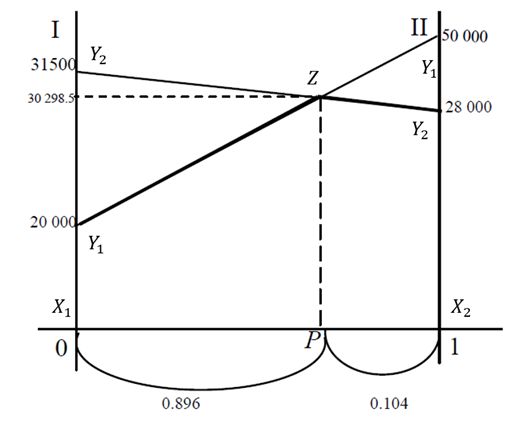
DOI: 10.9790/5728-1603030610 www.iosrjournals.org 8 | Page

A Cooperative Game Theory Application and Economical Behavior in an Aspect of Bangladesh …

 22− 12 28000 − 50000
 1 ∗ = = = 0.65
 11 + 22 − 12 − 21 20000 + 28000 − 50000 − 31500
And,
 2 ∗ = 1 − 0.65 = 0.35;
The value of the game is from (12) is:
 22 11 − 12 21 28000 × 20000 − 50000 × 31500
 = = = 30298.5
 11 + 22 − 12 − 21 20000 + 28000 − 50000 − 31500

 IV. Discussion
 The solution of the game means that AKS should mix its pure strategies, which consist of choosing the
 1 project jointly with RSRM with the probability 0.104 and the 2 project jointly with RSRM with the
probability 0.896. Project 1 together with GPH Ispat, AKS should choose with probability 0.65 and project
 2 with GPH Ispat, AKS chooses with the probability 0.35. Under these conditions, the expected gain will be
equal to the value of the game which is 30,298.5 BDT.
 This means that if AKS has to choose which strategy to follow, it would give preference to the
strategies with high probabilities. That is, 2 together with RSRM, and 1 together with GPH Ispat. These
results are summarized in Table 2. Note on the x-axis the segment with the length equal to one (Figure).
 The left part of the segment corresponds to strategy 1 and the right end corresponds to strategy 2 . All
the intermediate points of the segment correspond to the mixed strategies of AKS. The probability 1 = 0.104
of strategy 1 will be equal to the distance from point P to the right end of the segment, and the probability
 2 = 0.896 of 2 strategy is the distance to the left end of the segment. Let us draw two perpendiculars to the
x-axis through the points 1 and 2 axis I and axis II. The first will correspond to the gains that a firm could get
choosing strategy 1 and the second to strategy 2 .

 Table-2: Mixed strategy distribution for AKS
 Projects
 Competing firm
 1 2

 1 RSRM 1 ∗ = 0.104 2 ∗ = 0.896

 2 GPH Ispat 1 ∗ = 0.650 2 ∗ = 0.350

One can also give a clear geometric interpretation for the solution of the 2 × 2 game. Following the instructions
above one can get Figure:

Let us draw the lines which correspond to strategy 1 . The length of the segment 1 1 equals 11 = 20,000,
while the length of the segment 2 1 equals 12 = 50,000. Similarly, draw the lines which correspond to
strategy 2 .
 We need to find the optimal strategy P*, for which the minimum payoff of AKS will be maximized. To
do this, let us draw a bold line (Figure) which corresponds to the lower bound of winning if strategies 2 and 1
are selected, i.e. the kinked line 1 2 . This line includes all the minimum gains of AKS at any of its mixed

DOI: 10.9790/5728-1603030610 www.iosrjournals.org 9 | Page

A Cooperative Game Theory Application and Economical Behavior in an Aspect of Bangladesh …

strategies. It is obvious that the best possible minimum value in this example is at point Z, and generally
corresponds to the point where the curve that indicates the minimum payoff of AKS gets its maximum value.
The ordinate of this point is the value of the game and equals = 30,298.5 . The distance from the left end of
the segment 2 and the distance to the right end of thesegment 1 respectively, are equal to the probabilities of
strategies 2 and 1 . As a result, it should be said that after considering the theoretic entry situation we came to
the conclusion that for AKS the optimal solution would be to mix its pure strategies, i.e. while competing with
RSRM, the choose 1 project with the probability 0.104 and the 2 project with theprobability 0.896. Project 1
together with GPH Ispat, AKS should choose with probability 0.65 and project 2 with GPH Ispat, AKS
chooses with the probability 0.35. Under these conditions, the expected gain will be equal to the value of the
game which is 30,298.50 BDT. This means that if AKS has to choose which strategy to follow, it will give
preference to the strategies with high probabilities that is 2 together with RSRM, and 1 together with GPH
Ispat.

 V. Conclusion
 This paper gives a mild and gentle intro to cooperative game theory in the economy. Cooperative game
theory could be a structural, instead of procedural theory. It put up unsatisfying for business strategy whereas
the business strategy is usually distressed with what a firm does. Elementary terms and components of game
theory and also the most significant solution concepts are induced with some sample implementations. One can
see that game-theoretic models are often accustomed to the analysis of many interesting economical phenomena,
including legislative bargaining in the economy, conclusions to go to analysis about international business, and
formation of coalition governments in comparative economy.

 References
[1]. Cano-Berlanga (2017), Enjoying cooperative games: The R Package Game Theory.
[2]. Baskov O (2017), Bounded computational capacity equilibrium in repeated two-player zero-sum games.
[3]. Elena Yevsyeyeva, Olena Skafa (2016), Game Theory in Economics Education.
[4]. Varian Hal R. (2014), Intermediate Microeconomics: A Modern Approach. Eighth Edition. W. Norton & Company.
[5]. Albert Michael H, Nowakowski Richard J, Wolfe David (2007), Lessons in play: an introduction to combinatorial game theory.
 A. K. Peters, Wellesley.
[6]. Werner F., Sotskov Y. (2006), Mathematics of Economics and Business. Taylor & Francis e-Library.
[7]. Osborne, M. J. (2004), An introduction to game theory. New York: Oxford University Press.
[8]. Jamus Jerome Lim (1999), Fun, Games & Economics: An appraisal of game theory in economics.
[9]. John von Neumann and Oskar Morgenstern (1944), Theory of Games and Economic Behavior.
[10]. Cournot (1838), Competition and Cooperation Among Producers: Cournot Revisited.

 Md Obaidul Haque, et. al. "A Cooperative Game Theory Application and Economical Behavior in
 an Aspect of Bangladesh with a Real- Life Problem." IOSR Journal of Mathematics (IOSR-JM),
 16(3), (2020): pp. 06-10.

DOI: 10.9790/5728-1603030610 www.iosrjournals.org 10 | Page