A model of the U.S. food system: What are the determinants of the state vulnerabilities to production shocks and supply chain disruptions? - The ...

Center for Climate, Regional, Environmental and Trade Economics
 www.create.illinois.edu

 A model of the U.S. food system: What are the determinants of the state
 vulnerabilities to production shocks and supply chain disruptions?

 Noé J Navaa, William Ridleyb, and Sandy Dall’erbac

a
 Economic Research Service, U.S. Department of Agriculture, Kansas City, MO 64105, USA,
noe.nava@usda.gov
b
 University of Illinois at Urbana-Champaign, Center for Regional, Environmental, and Trade
Economics, wridley@illinois.edu
c
 University of Illinois at Urbana-Champaign, Center for Regional, Environmental, and Trade
Economics, dallerba@illinois.edu

 CREATE Discussion Paper ##-22-01
 February, 2022

Abstract: We adapt a Ricardian general equilibrium model to the setting of U.S. domestic agri-food trade
to assess states’ vulnerability to adverse production shocks and supply chain disruptions. To this end, we
analyze how domestic crop supply chains depend on fundamental state-level comparative advantages –
which reflect underlying differences in states’ cost-adjusted productivity levels – and thereby illustrate the
capacity of states to adapt to and mitigate the impacts of such disruptions to the U.S. agricultural sector.
Based on the theoretical framework and our estimates of the model’s structural parameters obtained using
data on U.S. production, consumption, and domestic trade in crops, we undertake simulations to
characterize the welfare implications of counterfactual scenarios depicting disruptions to (1) states’
agricultural productive capacity, and (2) interstate supply linkages. Our results emphasize that the
distributional impacts of domestic supply chain disruptions hinge on the extent of individual states’
agricultural productive capacities, and that the capacity for states to mitigate the impacts of adverse
production shocks through trade relies on the degree to which states are able to substitute local production
shortfalls by sourcing crops from other states.

Climate, Regional, Environmental and Trade Economics
65-67 Mumford Hall
1301 West Gregory Drive
Urbana, IL, 61801

1. Introduction
The tradeoffs between self-sufficiency versus reliance on external sources in meeting regions’ food
needs have long been understood; however, debates over how best to structure food supply chains
in order to maximize their resiliency continue to persist. Proponents of inward-oriented food
systems emphasize the benefits of self-reliance, and recent work by Biedny, Malone and Lusk
(2020) finds that in spite of the sharp polarization of American political attitudes, beliefs from
either end of the ideological spectrum tend to favor food systems founded on proximate supply
sources as the best means with which to promote food system resiliency.1 A common claim from
proponents of such approaches is that as the distance between regions and their food sources
increases, the disconnect between the adverse environmental consequences of food production
widens, hindering regulators’ efforts to internalize the negative externalities of agricultural
production (Clapp, 2015).2 Most recently, the challenges created for the U.S. food system from
the onset of the COVID-19 pandemic led to wasted production, increases in food prices, and
disruptions to key links in the food supply chain (Hobbs, 2020; Thilmany et al., 2020; Martinez,
Maples, and Benavidez, 2021). Other recent disruptions to both international and domestic supply
chains have highlighted their susceptibility to disruptions at critical points in the system. For
instance, the upending of global trade networks caused by the recent temporary closure of the Suez
Canal illustrated how disruption at a single critical point can cause widespread disruption, while
at the domestic level, food prices can potentially raise due to this short-run fall in supply.
 In contrast, economists have long emphasized the ways in which specialization and
interdependence through trade can facilitate access to efficiently produced products (Krugman,
1981; Eaton and Kortum, 2002; Arkolakis, Costinot, and Rodríguez-Clare, 2012) and promote
resiliency in the food system (Reimer and Li, 2009, 2010). Classical theories of trade and
specialization make clear that food systems will be most efficient when they allow for regions to
exploit differences in comparative advantage. Perhaps most importantly, the permanent
availability of external food sources ensures that disruptions to local supply can be mitigated
through reliance on trade partners (Ferguson and Gars, 2020; Dall’Erba, Chen, and Nava, 2021).

1
 Proponents of policies that promote local agriculture also raise environment and health concerns in
addition to concerns relating to the resiliency of outward-oriented food systems emphasizing reliance on
distant sources of supply (DuPuis and Goodman, 2005; Levkoe, 2011; Marsden, 2013).
2
 In Blay-Palmer et al. (2013), several examples of bottom-up approaches to the promotion of local
agriculture are discussed.

Therefore, while inward-oriented food system approaches emphasize the disadvantages of reliance
on distant supply sources, outward-oriented strategies for food system design tend to highlight the
benefits arising from trade and specialization alongside the capacity of such systems to mitigate
the impacts of negative shocks to one’s own production through interdependence and trade.
 Due to the complexity of the U.S. food system and the importance of domestic supply and
demand relationships in U.S. agriculture, the optimal design of the food system necessitates an
appraisal of inter- and intra-state reliance in order to assess the advantages and disadvantages of
each. However, while a broad assortment of work has addressed these issues in appraising food
systems at the international level (Grant, and Lambert, 2008; Reimer and Li, 2009, 2010; Martin,
2018), a paucity of work on food systems and trade relationships at the domestic level prevents
researchers from analyzing these same important questions of resilience and efficacy (Smith et al.,
2017; Lin et al., 2019). In this paper, therefore, we undertake a quantitative analysis of the U.S.
domestic food system by adapting a structural, general equilibrium model of trade based on
Ricardian comparative advantage and gravity relationships to U.S. states’ supply and demand for
primary crops in order to quantify the efficacy of various strategies in promoting food systems’
efficiency and resilience.
 An ideal approach with which to jointly consider supply, demand, and trade relationships
between regions is the gravity model, in which bilateral trade is expressed as a function of the size
of supply and demand in the exporter and importer, respectively, and both bilateral and multilateral
barriers to trade. Approaches based on gravity models are ideal for assessing the welfare and
consumption implications of various policy counterfactuals in that they are theoretically founded
and can be derived based on either demand-based (Anderson, 1979; Bergstrand, 1985; Anderson
and van Wincoop, 2003) or supply-based (Chaney, 2008; Chor, 2010) formulations. In settings
where regions’ productivities – and thus, their comparative advantages, and the scope for
specialization and interdependence – are the central focus, supply-side analyses offer the ideal
approach with which to assess the resilience and efficiency of trade networks. Along these lines,
the seminal work of Eaton and Kortum (2002) (henceforth, EK) develops a model which considers
the producers’ relative comparative advantages as reflected by differences in cost-adjusted
fundamental productivities, and which further yields a tractable framework with which to
empirically assess welfare, consumption, and trade under alternative counterfactuals. We therefore

 1

adapt the theoretical framework of EK to the setting of the domestic U.S. trade in crops in order
to analyze and explore the properties of the U.S. food system.
 Despite its widespread use in the broader trade literature, only a few empirical studies of food
and agriculture base their analyses on a Ricardian notion of comparative advantage. Similar to our
work is that of Reimer and Li (2009, 2010) that exploit this formulation at the international level
to study how yield variability across countries determines the welfare of consumers, finding that
openness to trade increases countries’ welfare whenever they experience adverse yield conditions.
Recent work by Heerman (2020) incorporates agro-ecological conditions into the Ricardian setting
as a determinant of productivity, while Devadoss, Ugwuanyi, and Ridley (2021) augment the
Ricardian setting with Heckscher-Ohlin-style endowment effects. In a similar fashion, we adapt
and estimate the EK model in order to study U.S. states’ food vulnerability in the existing domestic
food system and to assess the efficacy of the system under various policy counterfactuals.
 To analyze these issues, we consider two distinct counterfactual scenarios. First, the impacts
of shocks to individual states’ productivities are simulated as arising through reductions in each
state’s agricultural capacity – a structural parameter (described in detail below) that governs each
state’s agricultural productivity. Second, food supply chain disruptions are modeled by
significantly increasing the costs of interstate trade between each pair of states. To assess the
distributional impacts under these various counterfactuals, we construct a ranking of relative
comparative advantage to pinpoint how states’ underlying relative productivity levels as a key
determinant of food vulnerability in each of our simulations. We find that the distribution of
welfare losses depends on each state’s ability to substitute consumption sources, which depends
on both its own fundamental productivity and on its ability to efficiently source crops from other
states.
 Our work makes three primary contributions to the literature on food security and trade. First,
our approach is based on a comprehensive but tractable model of the U.S. market for crops that
can be employed to analyze a large array of counterfactuals concerning food security in the United
States. This approach accounts for the heterogeneity of farmers’ productivities by incorporating
and estimating producer-specific efficiency terms. In addition, we recognize food processors and
other intermediate users as the main consumers of farmers’ production and isolate their substitution
effect. Secondly, we construct a state-level ranking of relative comparative advantage using data
on domestic interstate trade. While most Ricardian trade studies recognize competitiveness (i.e.,

 2

the exporter’s relative cost-adjusted productivity) and openness (i.e., the importer’s relative ease
of access to externally sourced products) in their applications, researchers do not exploit the
ranking and rather focus on the decomposition of the determinants of productivity and comparative
advantage. We use this ranking of relative comparative advantage in the U.S. food system to study
the mechanisms that shape welfare losses in our food vulnerability counterfactuals.
 Due to the challenges associated with collecting domestic trade data, our third and final
contribution relates to expanding the body of work analyzing trade in domestic settings, a literature
that remains nascent in spite of the profound importance of domestic trading relationships in the
United States and elsewhere. One benefit afforded by this setting is that U.S. domestic trade is
absent of non-market barriers such as tariffs, and focusing on domestic trade thereby presents the
opportunity to study the market mechanisms that govern trade and welfare distributions absent of
policy confounders. To our knowledge, our study is the first to adopt a general equilibrium
Ricardian approach to modeling productivity and domestic trade in agriculture at a regional (sub-
national) level in a modern setting.3
 The remainder of the paper is organized as follows. The next section describes our extension
of the formulation of EK, and its implications for the U.S. domestic market for crops. Section 3
presents our empirical strategy. First, we describe how we process the data to capture the economic
realities of the U.S. domestic crop market. We then econometrically estimate the structural model
parameters necessary for our post-estimation simulations and conduct a decomposition of each
state’s comparative advantage. In section 4, we describe our simulation strategy and then present
and discuss the results from our counterfactuals. Finally, we offer concluding remarks in section
5.

2. A Ricardian trade model of U.S. domestic crop production
As described earlier, we adapt the canonical EK formulation to the setting of domestic U.S. crop
trade in order to assess how welfare, production, and consumption respond to disruptions in the
U.S. domestic food system. In this section, we recount the key features of the EK model and
describe how its components correspond to the U.S. domestic system, and how the modelling
framework will allow us to (1) tie the model’s equilibrium relationships on production,

3
 Donaldson (2018) employs a Ricardian model of agricultural productivity and sub-national trade in the
context of colonial India.

 3

consumption, trade, and welfare to observed data, and (2) empirically estimate the model’s
fundamental parameters in the setting of U.S. domestic trade in crops.
 On the supply side, we denote producers (farmers) by i and refer to them as exporters,
producers and the origin of the commodity interchangeably. Producers operate under different
weather, technology and land characteristics across U.S. states.4 We capture their heterogeneity
with a land productivity term denoted as ( ), where l indicates commodity (with ∈ [0,1]), a
technological productivity-augmenting factor denoted as , and farmers’ production costs denoted
as (Eaton and Kortum, 2002; Heerman, 2020). We denote final prices as ( ) and bilateral
trade costs as . They distinguish the source of the commodity i and the location of consumption
j5. Assuming constant-returns-to-scale technology and perfectly competitive output and input
markets, the final price is related to costs of production, the producer’s efficiency, and bilateral
trade costs as given by:
 
 ( ) = . (1)
 ( ) 

The producer-specific productivity term, , is assumed to be drawn from a Fréchet probability
 − 
distribution, ~ ( ) = − . Here, > 0 is a producer-specific parameter that governs a
region’s productivity outcome, so as grows larger, the probability of drawing a large value for
the idiosyncratic efficiency outcome increases. We refer to as agricultural capacity. The
parameter > 1 is common across producers and governs the dispersion of the productivity draws
of individual producers. As tends to infinity, the probability of any individual region maintaining
a large comparative advantage decreases (i.e., large values imply that productivity differences
between regions will be minimal and differences in regions’ comparative advantages will therefore
be small). The employment of the Fréchet distribution is a realistic approach since its quality of
focusing on extreme values captures both individual producers’ productivity and the overall
distribution of comparative advantages across all producers.

4
 A vast existing literature analyzes the heterogeneity of farmers’ responses to weather and climate
conditions. Starting with their canonical Ricardian approach, Mendelsohn, Nordhaus and Shaw (1994)
forecast that climate change will create winners and losers in U.S. agriculture depending on the best use of
farmers’ land. Cai and Dall’erba (2021) offer a review and a test of the more recent contributions that add
heterogeneous producers’ resilience to weather shocks depending on geographical location.
5
 Bilateral trade costs are modeled in a multiplicative (“iceberg”) fashion and assuming that there are no
intra-region trade costs (i.e., = 1).

 4

In turn, we consider food processing plants and other intermediate users of crops as the
demand side (as final household demand comprises a comparatively small share of primary crops’
use in the United States). We index these intermediate users by j, and we refer to them as importers,
consumers and the destination of the commodity interchangeably. Consumers utilize farmers’
crops according to a CES technology depicted in Equation (2):
 − 
 1 −(1− ) (1− )
 ( ) = [∫0 ( ) ] , (2)

where > 0 is the elasticity of substitution, and ( ) denotes the quantity of good l consumed
by j from source i. For simplicity of notation, we omit l from the rest of the description of the
model.
 Next, the Fréchet distribution, Equation (1), and Equation (2) are combined to retrieve a
 − 
distribution of final prices: ( ) = 1 − −Φ . Here, Φ = ∑ ( ) , where I denotes the
set of all producers, ultimately connects all regions’ technologies, production costs and bilateral
trade costs into the final price faced by purchaser j. This relationship is illustrated in Equation (3):
 1
 − − 
 = [∑ ( ) ] , (3)
 +1− 
where γ = Γ ( ) and Γ is the gamma function. The model thus captures a market where each
 
profit-maximizing producer offers a different price to each expenditure-minimizing consumer
determined by the producer’s technology/productivity parameter in conjunction with unit
production costs and trade costs . In turn, the intermediate user possessing the production
technology expressed by Equation (2) sees all prices and chooses the lowest one. Therefore, the
allocation of commodities reached by the producers and consumers yields the market equilibrium
illustrated in Equation (3).
 To empirically consider equilibrium deviations and their welfare consequences, the structural
parameters , , and are connected with information on production, consumption, and bilateral
trade between regions. Let = ∑ be region j’s expenditures on commodities from all regions,
where is the value of trade going from i to j (including j’s purchases from itself). The
distribution of prices introduced earlier implies that the fraction of a state’s expenditure on crops
from any state i is equal to the probability that the state i offers the lowest price. Thus, trade shares
are connected to the structural parameters as seen in Equation (4):

 5

− 
 ( )
 = − . (4)
 ∑ ( )

 Equation (4) has two empirical properties regarding short-run substitution behavior in the
face of extreme weather events6. By simulating a region’s decline in crop yields through a
reduction in the value of , Equation (4) implies that if a region is impacted by some adverse
shock to its production (for instance, adverse weather conditions during the growing season), the
region will be obliged to rely more on imports. On the other hand, if the shock to production affects
instead any of the region’s import sources, then the region will import less from the affected
producer7.
 Because crop production combines several inputs, we assume that harvesting a given land
area utilizes the operating inputs labor and land together with intermediate inputs (e.g., seed and
fertilizer) based on a Cobb-Douglas function:
 1− 1− 
 = ( 1− ) = λ , (5)
where is the wage rate, is the land rental rate, is the share of operating expenses from labor
and land inputs (denoted ), and is the labor and land share of production costs. reflects the
price index for intermediate inputs, which comprise a share of production costs equal to 1 − .
 
We additionally normalize Equation (4) by multiplying it by domestic sales, ( ), and thus obtain
 
Equation (6). A final step that allows for relative prices to be eliminated from the model (and
therefore for regions’ consumption shares to thus be expressed as a function of operating expenses,
fundamental productivity levels, and trade costs) involves combining the expression for
intermediate use with Equation (3) into Equation (6):
 − − (1− )
 − 
 = ( ) ( ) , (6)
 
which thereby generates the trade-share equation which will be the relationship of primary interest:

6
 Let = / . Then ∂ / ∂ < 0, i.e., there is an inverse relationship between region j’s expenditures
on goods from producing region i and the level of j’s agricultural capacity. Further ∂ / ∂ > 0, i.e. there
is a positive relationship between region j’s expenditure on goods from producing region i and the level of
i’s own agricultural capacity.
7
 Dall’erba, Chen and Nava (2021) provide empirical evidence of producers substituting domestic
intermediate inputs for imports when U.S. states are impacted by drought events.

 6

1
 ′ 
 λ 
 ′ = ( ) ( 1 ) 
 − 
 , (7)
 λ 
 
 (1− ) 
where the logarithm of the left-hand side is given by ln ′ = ln − [ ] ln ( ) and ln ′ =
 
 (1− ) 
ln − [ ] ln ( ), which is defined as normalized trade.
 
 Equation (7) is a version of the gravity equation expressed in terms of expenditure shares
rather than absolute trade volumes, in which the expressions in parentheses are the size terms8. In
contrast to gravity equations derived from the demand side, normalized trade depends primarily
on the regions’ comparative advantages arising from differences in cost-adjusted productivity
levels. For example, the size term associated with the exporter increases as the exporting region
becomes more productive (i.e., increases), but decreases as the exporting region’s production
expenses rise (i.e., λ increases). The technology-expense relationship is inverted for the importer.
The more expensive it is for an importer to produce due to high inputs prices (i.e., λ increases),
the more the region is likely to rely on imported consumption. In contrast, the more productive a
destination region becomes (i.e., increases), the greater is the region’s reliance on domestic
production.
 Having established the relationship characterizing the determinants of bilateral trade, we
can define our welfare measure as changes in consumers’ real expenditure on crops. First, each
region’s aggregate expenditures can be obtained as = , where is the number of harvested
acres in i. Thus, Equation (4) can be manipulated to analyze a region’s income through Equation
(8):
 − 
 ( )
 = ∑ − . (8)
 ∑ ( )

Using hat-algebra, which allows us to specify the model in terms of changes from the equilibrium
(Dekle, Eaton and Kortum, 2007), we define a measure of changes in regions’ equilibrium
expenditures that arise from changes in the structural elements such as production costs ( ),
fundamental productivity ( ) and trade costs ( ) as given in Equation (9):

 1/ 
8
 A further re-arrangement of the equation’s components allows us to define and as multilateral
resistance terms (as discussed in Anderson and van Wincoop (2003) and others) that inhibit trade between
the two regions.

 7

− 
 ̂ 
 ̂ = ̂ ̂ − ∑ ̂
 , (9)
 ∑ ̂ ̂ − 

 ′
where the hat notation describes relative changes in a variable’s value. Thus, ̂ = is the change
 
 ′
in farmers’ operating expenses per harvested acre, ̂ = is the change in agricultural capacity,
 
and ̂ is the change in expenditure. = is a bilateral trade/expenditure share that indicates
 
how much of j’s expenditure comes from i in the baseline equilibrium. Changes in trade costs are
expressed as ̂ − = , where = 0 if no change in bilateral trade costs is analyzed.
 ̂ + 
 Finally, we define consumers’ change in nominal expenditure in state i as ̂ = ,
 
where is an additive component to account for trade imbalances (since we assume, as in EK,
 ̂ =
that trade is balanced). Then, nominal expenditure change is normalized by change in prices: 
 −1/ 
[∑ ̂ ̂− 
 ] in order to express welfare impacts under various counterfactuals in terms of
changes in real expenditures. Therefore, Equation (9) is reduced into our final expression for
 ̂ is the change of welfare in i:9
welfare given by Equation (10), where 
 ̂
 ̂ = .
 (10)
 ̂ 

 The welfare impacts of disruptions that affect farmers’ production can be studied by
solving the previous system of equations with simulated values for ̂. Similarly, we can study
perturbations to bilateral trade costs, such as those caused by disruptions in the food supply chains
between states, with simulated values for ̂ − 10.

3. Empirical Strategy
In this section, we first discuss the databases and the data treatment employed in our analysis. We
then use these data to recover the necessary structural parameters to conduct our simulations in a
two-step approach. The final sub-section describes the implied relative comparative advantages of
U.S. states in the domestic market for crops.

9
 Because our welfare measures are defined in terms of changes in real expenditures, welfare measures can
be comparable across U.S. states. The theoretical model of EK models regions as representative consumers,
which can be thought of as the average consumer in each region. In that sense, the average consumer in a
U.S. state can be compared with that of another state.
10
 The system of equations described here can be easily solved using the tools provided in Baier, Yotov,
and Zylkin (2019) and the Stata statistical software.

 8

3.1 Data
U.S. crop markets are comprised of multiple producers with heterogeneous production
technologies, but there are only three major consumers of U.S. crops: food processors and other
intermediate users that buy crops for processing, exporters that resell U.S. domestic production
overseas, and households that buy unprocessed crops such as fruits and vegetables. This distinction
has empirical implications, as substitution effects (i.e., in Equation (2)) are likely to be different
depending on the type of demand. For example, exporters’ demand for domestic crops is
determined by international consumers, while food processing plants’ demand for domestic crops
is an intermediate step in the mainly domestic food supply chain.
 To homogenize consumption and to account for the substitution effects between crops
varying across different domestic purchaser groups, we drop foreign trade from our analysis. One
concern that might arise is that such a restriction limits the comprehensiveness of our analysis of
crop production. We study whether our modelling decision is a limitation using our main dataset,
the U.S. Freight Analysis Framework (FAF4). FAF4 contains aggregates of crops as classified by
the Standard Classification of Transported Goods (SCTG), based on national-level input-output
relationships. SCTG 02 refers to the crop aggregation comprising cereals and grains, while SCTG
03 encompasses fruits, vegetables, oilseeds such as soybeans, and a handful of other assorted
primary food crops. The share of U.S. crop production that is exported is roughly 10% with the
largest part being SCTG 02. In addition, our conceptual mathematical model developed in the
previous section characterizes food processing plants as the main consumer of farmers’ crops.
Only 12% of U.S. crop production goes directly to households, and therefore the large majority
of primary U.S. crop production goes to domestic intermediate uses.
 The Bureau of Transportation Statistics (BTS) and the Federal Highway Administration
(FHWA) developed the FAF4 data in an effort to impute domestic data flows between all U.S.
states (including intra-state flows, i.e., states’ trade with themselves) for several commodities and
is based on the BTS Commodity Flow Survey (CFS) for most types of commodities; however,
because the CFS treats goods transported by agricultural firms as outside of its scope, the FAF4
dataset uses information from the U.S. Department of Agriculture’s Census of Agriculture to more
accurately model the true extent of domestic trade flows in farm products. Our measure of crop
trade flows is constructed by aggregating SCTG 02 (cereal crops) and SCTG 03 (fruits and

 9

vegetables, and a handful of other crops such as soybeans). We confine our focus to the lower 48
U.S. states, as Alaska and Hawaii are not large agricultural producers and face a significantly
different trading environment relative to contiguous U.S. states.
 Table 1 describes the data for each of the variables used in our analysis. The top part of the
table describes dyadic variables that capture attributes about the relationship between two states.
Here, we consider geographical distance and whether two states share a contiguous border, two
standard measures of geography-based trade costs from the gravity literature (Larch and Yotov,
2016). To measure the distance between any two states (in kilometers), we calculate the distance
between the states’ centroid in a shapefile using the Geoda software. The bottom part of the table
describes monadic variables that capture attributes specific to individual states that will be used to
estimate the comparative advantage dispersion parameter . Imports and exports are created using
FAF4 data to describe trade flows. Both measures are in millions of 2017 U.S. dollars. Population
density, which we will use as an exogenous predictor of operating costs in an instrumental variable
analysis below, is collected from the 2010 U.S. Census Bureau of Statistics and is measured in
population per square kilometer. Operating expenses per harvested acre are obtained from the 2017
U.S. Census of Agriculture and are measured in 2017 dollars. Climate variables that affect
agricultural output during the Summer are precipitation and temperature during summer.
Precipitation is measured in cubic centimeters, and temperature is measured in degrees Celsius.
Weather data are collected from the Parameter-elevation Regression on Independent Slopes Model
(PRISM) data base over the 20 years period between 1997 and 2017. Then, weather data are
transformed into climate by taking the average of each variable over time for each location
(PRISM, 2011).
 Because virtually all agricultural activity occurs outside cities and our climate variables
described earlier could be influenced by urbanization, we follow a two-step aggregation of our
data variables. First, all data are obtained at the county level for all counties in the contiguous
United States. Next, metropolitan and highly populated counties are dropped (Dall’Erba and
Dominguez, 2016)11. Finally, we calculate state averages excluding metropolitan and high
population counties. This aggregation technique allows us to reduce weight from highly populated,
urbanized regions with little agricultural production.

11
 We define the population density cutoff at the county level is 1,600 persons per square mile.

 10

Table 1: Trade, crop operating expenses, population density and climate variables in 2017
 Dyadic Variables Mean S.D. Min Max
 Distance 1827.27 1295.40 0.00 5179.18
 Contiguity 0.10 0.29 0.00 1.00
 Monadic Variables Mean S.D. Min Max
 Imports 9,280.78 9,934.75 233.99 43,387.97
 Exports 9,280.78 10,927.41 105.50 46,177.39
 Operating expenses per harvested acre 708.75 492.77 75.83 2478.09
 Population density 83.85 61.69 6.46 286.11
 Summer temperature 24.25 3.70 18.27 32.30
 Summer precipitation 42.27 16.68 3.33 82.93
 Notes: The number of observations for our dyadic variables is 2,304, while the number of observations
 for our monadic variables is 48. All monetary measures are in 2017 U.S. dollars. The value of imports
 and exports are created using FAF4. Distance is measured in kilometers. Population density is measured
 in population per square kilometers. Precipitation is measured in cubic centimeters, and temperature is
 measured in degrees Celsius.

3.2 Recovering Structural Parameters
Recovering the structural parameters and requires a two-step approach. First, Equation (7) is
parameterized with the log-linearization of the expression. Equation (12) is the regression model,
where the size terms are denoted by for the exporter and for the importer and are captured
through the use of importer and exporter fixed effects. The error term is . Then, size term
estimates are used in a second-step as the dependent variable in the estimation of Equation (13),
where the size terms come from Equation (7) and are denoted as ̂ and ̂ for the exporter and the
importer respectively:
 ′
 
 ln ′ = − ln + − + , (12)
 
 1
 ̂ = + ln − ln + , (13)
 
where is the error term. In contrast with Equation (12), in which is attached to a variable ( )
that is difficult to directly measure empirically, can be recovered from Equation (13) since it is
associated with an observable variable ( , or operating expenses). We assign a value of 0.12 to
the share of intermediate inputs (1 − ) based on input-output data from IMPLAN12. The

12
 We consider 1 − = 0.12, the weighted average of intermediate-input shares in our crop aggregations
for SCTG02 and SCTG03 (for example, fruits and vegetables), acknowledging that some crops in our
aggregation require higher operating expenses because of differences in labor and/or land intensity in
production. For robustness, we consider the impact of alternative assumptions on for our simulation
results, and find that values in the range 1 − ∈ [0.08, 0.21] generate qualitatively similar results in our
counterfactual simulations.

 11

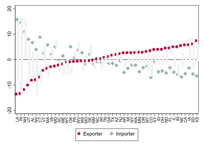
estimation of Equation (12) is carried out through the use of dummy variables. Since bilateral trade
costs are not readily observable, we approximate them through the use of two variables reflecting
geographical determinants of trade costs: a contiguity dummy that indicates whether two states
share the same border and six dummies corresponding to the distance bins (0, 865], (865, 1730],
(1730, 2595], (2595, 3460], (3460, 4325] and (4325, Max]13. Since we assume that intra-trade has
zero cost (i.e., = 1), then all dummies for distance are interpreted relative to intra-trade costs.
Importer and exporter fixed effect dummy variables are included, but normalized to sum to zero.
Notice that the estimation of Equation (12) will drop all zero-trade observations (i.e., = 0).
Because trade between regions is not symmetric, the variance-covariance matrix is assumed to
have diagonal elements 12 + 22 that affect both two-way trade and one-way trade, and certain
nonzero off-diagonal elements 22 that affect only two-way trade. For this reason, we estimate
Equation (12) by feasible generalized least squares14 (FGLS).
 Figure 1 reports estimates from Equation (12). In panel (a), we report the proxy estimates
for bilateral trade costs (using trade data aggregated across the two SCTG commodity groupings).
As expected, two states sharing a contiguous border tends to be associated with more trade between
the states. Our results indicate also that trade volumes decrease with distance, but the marginal
impact of distance on trade becomes attenuated in the last two distance bins. We attribute this to
freight mode decisions. Our FAF4 data shows that while most crops are shipped within short
distances by truck, the volume shipped by truck decreases with distance but increases for rail and
barges, modes for which long distances incur only small marginal transportation costs.
 In panel (b), estimates of the fixed effects are depicted graphically. The estimates
associated with the size terms are structurally symmetric as shown in Equation (7). Deviations
from symmetry represent non-market influences that affect either the imports or exports from a
region. For instance, as described earlier, each set of fixed effects can be interpreted as either
competitiveness or openness for the exporter and importer side respectively. In an international
trade context, this distinction typically reflects institutional and policy differences that affect

13
 Using distance bins, as supposed to a continuous distance measure, allows us to assign no ad-hoc
parametrization to Equation (12). No significant difference is found when using a continuous measure of
distance when running Equation (13).
14
 Recent papers that estimate Equation (12) report employing versions of the Poisson pseudo-maximum
likelihood (PPML) estimator to address the heteroskedasticity and zero-trade issues. In our two-step
estimation to estimate , we do not advise the employment of PPML since the second step, Equation (13),
is a linear estimator.

 12

specific countries, such as weak government institutions, which impact exports, and policies that
encourage citizens to consume domestically sourced goods, which affect imports. We test for
symmetry of the fixed effect estimates by testing the difference between each pair of estimates.
Furthermore, the imposed symmetry of our structural model prevents us from testing whether point
estimates are statistically different from zero since each set of size-term fixed effects crosses zero.
For this reason, the symmetry test also serves as a significance test. The point estimates are shown
without confidence intervals, but the confidence interval corresponding to the test of whether each
pair is equal to each other is shown.
 Figure 1: Estimation results from gravity equation: Distance and importer- and exporter-size
 effects.

 (a) Bilateral trade costs (b) Size terms
 Note: R2 is 0.97 with 1,334 observations. The imposed symmetry of our structural model
 prevents us from testing whether point estimates are statistically different from zero since each
 set of size term fixed effects crosses zero. For this reason, we instead test whether the absolute
 values of point estimates in each pair of size terms is equal to each other. The point estimates
 are shown without confidence intervals, but the confidence interval for the test of whether each
 pair is equal to each other is shown.

 Using estimates for the size terms, we estimate Equation (13) to recover . Since
agricultural capacity ( ) is not observed, we proxy it using historical precipitation and
temperature for each U.S. state, following a quadratic polynomial with an interaction term.
Because we expect high operating expenses per acre to be associated with high levels of
agricultural capacity (e.g., high operating expenses might be indicative of a region having more
productive soil, and thus higher levels of demand for inputs), we employ the two-stage least
squares (2SLS) estimator. Our instrumental variable is average population density in rural counties
within each U.S. state. We expect that the wage component in Equation (5) is affected by
 13

population density, so our use of this variable ensures that our instrument affects operating
expenses per acre, but not other determinants of agricultural capacity such as climate15.
 Table 2 reports the results from the estimation of Equation (13). The exporter columns use
the size terms related to the exporter, and the importer columns use the size terms related to the
importer. The first column employs the OLS estimator and the second column the 2SLS estimator.
The variance inflation factors of the climate variables are above 100 in every regression, so the
climate estimates are highly correlated16. Our conceptual framework predicts to be positive and
greater than 1, so the coefficient associated with operating expenses per harvested acre must be
negative and less than 1. The results from the OLS estimations show that is not statistically
different from zero. As expected, correcting for endogeneity leads to larger and statistically
significant estimates of , which again reflects the notion that unobserved aspects of productivity
might be correlated with operating expenses. The specification based on the exporter size terms
yield an estimate = 2.962, while the estimates obtained by using the importer size terms
generate a slightly larger value of = 3.804. Table 2 also reports the first stage and allows us to
reject the hypothesis that our instrument is weak17.
 We compare our estimates of the comparative advantage dispersion parameter with those of
Reimer and Li (2010) who estimate this parameter for crop yields at the international level. Their
point estimates for are no lower than 2.52 and no higher than 4.96. Using a generalized method
of moments approach, they estimate = 2.83 compared to a value of = 2.52 using maximum
likelihood and a parametrization of the Fréchet distribution. The authors also report a larger
estimate of at 4.96 based on using the relative prices of the commodities under consideration to
proxy for elements of the EK model. However, Simonovska and Waugh (2014) show that the use
of such proxies can systematically generate overestimates . Therefore, because our importer side

15
 The threat to the exclusion restriction when population density is the aggregate of the whole state is that
climate change is affected by activities related to population density such as traffic and polluting industries,
which are typically concentrated in cities and their surrounding areas. Our instrument is weakly and
negatively correlated with temperature in the growing season. In fact, a large part of the variation in
agricultural productivity is explained by climate and land characteristics, ensuring that population density
only affects operating expenses per harvested acre (Liang et al., 2017).
16
 Because the coefficient of interest is , climate proxies are simply used as control variables.
17
 A concern associated with the estimations in Table 2 is the finite sample properties of the IV estimator
(Heid, Larch, and Yotov, 2017). Andrews and Armstrong (2017) report that exactly identified models with
low number of observations often possess undesirable properties (such that the IV estimator is consistent
but not unbiased), but the authors propose an estimator that is unbiased. We implement their estimator and
find no difference with the estimations in Table 2.

 14

Table 2: Second step estimations, using OLS and 2SLS estimators
 Exporter Importer
 OLS 2SLS OLS 2SLS

 Labor expenses –0.008 –2.962** –0.497 –3.804***
 (1.138) (1.344) (1.175) (1.399)
 Temperature 2.643 2.301 3.433 3.049
 (2.899) (2.968) (2.995) (1.399)
 Precipitation –0.167 –0.032 –0.136 0.015
 (0.325) (0.313) (0.336) (0.315)
 Temperature2 –0.056 –0.044 –0.068 –0.055
 (0.058) (0.054) (0.059) (0.054)
 Precipitation2 –0.001 0.001 0.001 0.002
 (0.003) (0.003) (0.003) (0.003)
 Interaction 0.007 –0.001 0.002 –0.008
 (0.015) (0.018) (0.016) (0.018)
 Constant –29.864 –10.245 –36.514 –14.545
 (37.515) (37.750) (38.748) (37.9423)

 First Stage
 Population Density 0.709*** 0.709***
 (0.085) (0.085)
 F Statistic 14.81 14.81
 R2 0.10 0.59 0.08 0.59
 Observations 48 48 48 48
 Notes: *** p < 0.01, ** p < 0.05, * p < 0.10.
 Operating expenses and population density are natural logarithm values. Coefficient associated
 with operating expenses is . Values in parentheses are robust standard errors. Coefficients for
 1
 climate variables are recovered up to the constant .
 
estimate of = 2.962 falls squarely in the range of estimates found by Reimer and Li (2010), we
choose it as our preferred value for the comparative advantage dispersion parameter because it
closely approximates existing values of this parameter from the literature.

3.3 Comparative Advantage
To analyze the comparative advantage of each U.S. state, Equation (13) is re-arranged into the
 
relationship ̂ = ( ̂ ) , which expresses agricultural capacity as a function of parameters, the
estimated size terms, and operating expenses. Using data on operating expenses per harvested acre,
the estimates for the exporters’ size term, our preferred value for = 2.962, and = 0.88, we
calculate the value of each state’s agricultural capacity. Thus, each state’s exporter size terms can

 15

be decomposed into an agricultural capacity component and an operating expense component. This
decomposition is shown in Figure 3.
 Figure 2: Comparative advantage (exporter size-term) decomposition

 Note: Figure reports size terms estimates obtained using Equation (13): natural log of the
 implied level of agricultural capacity and natural log of operating expenses per harvested acre
 in each U.S. state multiplied by = 2.962. Implied level of agricultural capacity is calculated
 
 as ̂ = ( ̂ ) .

 All else constant, Equation (7) implies that net exporters have high levels of agricultural
 1/ 
capacity relative to their operating expenses ( > λ ). This is because regions with relatively

high levels of agricultural capacity relative to their input costs are better able to specialize in crop
production. Similarly, net importers have low levels of agricultural capacity relative to their
 1/ 
operating expenses ( < λ ). Therefore, the size term can be interpreted as a state’s
comparative advantage. Figure 3 shows that a state’s comparative advantage largely depends on
its agricultural capacity. While operating expenses per harvested acre typically fall within a
relatively narrow range of values, agricultural capacity can take extreme values. Further, as
implied by the model, states with high agricultural capacity relative to operating expenses are
predicted to be net exporters based on comparative advantages maintained over other states.

 16

Our results indicate that Kansas, South Dakota, Iowa, California, Nebraska, Indiana, Illinois
and Florida have a comparative advantage in the U.S. market for crops. Not surprisingly, these
eight states jointly account for over half of all U.S. domestic crop production. However,
comparative advantage in crop production is not only determined by agricultural capacity.
Agricultural capacity is largest for California and Florida, but their comparative advantage is
dragged down by high operating expenses within the state. This emphasizes the importance of
reducing operating expenses to compete. On the other hand, Louisiana, Rhode Island, New
Hampshire, Utah, Alabama and Nevada have the lowest levels of agricultural capacity and high
operating expenses. These six states export less than 2% of domestic crop production and import
up to four times what they export.

4. Food vulnerability simulation results
We next turn to employing the estimated structural parameters that reflect the states' comparative
advantages and our data on domestic crop trade to conduct two counterfactual simulations. The
first simulation is designed to assess the U.S. states’ vulnerability to food supply chain disruptions.
This scenario considers an increase in bilateral trade costs separately (i.e. = 1.5 ∀ ≠ ) for
each state to quantify the degree to which individual states are vulnerable to food supply
disruptions. While the state’s comparative advantage can help mitigate welfare losses caused by
supply chain disruptions, we conduct an additional simulation to investigate the ability of the
existing food supply chain to mitigate welfare losses from events that affect each state’s ability to
produce crops (i.e., = 0.5 ∀ ). The numerical results on the key outcomes for each of our
simulations are shown in Table 3 and further describe in Figure 3 and Figure 4. Notice that we
decompose our welfare measure into a total expenditure term, ̂ , and a price index term, 
 ̂ , so our
welfare measure is real expenditure for crops (Arkolakis, Costinot, and Rodríguez-Clare, 2012).

 17

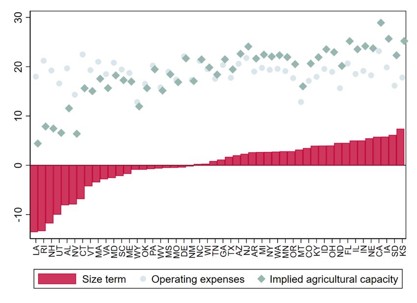
On average, both simulations produce welfare losses around 15%, but divergence in
counterfactual expenditure and prices signals the mechanisms that govern each simulated event.
Our supply chain shock results indicate that expenditure fall by 16% with a small hike in the level
of prices. The latter effect suggests that the primary factor governing welfare losses from
disruption of supply chains in the U.S. is shortage of crops. Recent literature (Ferguson and Gars,
2020; Dall’Erba, Chen, and Nava, 2021) provide empirical evidence of producers substituting
domestic intermediate inputs for imports when U.S. states are impacted by drought events. Results
in the bottom part of Table 3 investigate the capacity for states to mitigate impacts of adverse
production shocks through trade. In contrast to our initial simulation, our production shock
 Table 3: Simulation results
 Supply chain shock
 Mean Std. dev Minimum Maximum
 ̂ 
 0.82 0.072 0.66 0.96
 ̂ 0.84 0.069 0.67 0.96
 ̂ 
 1.02 0.010 1.01 1.05
 Production shock
 Mean Std. dev Minimum Maximum
 ̂
 0.89 0.081 0.71 0.99
 ̂ 1.12 0.038 1.04 1.19
 ̂
 1.27 0.107 1.07 1.45
 Notes: Table shows descriptive statistics from simulation results for all
 U.S. states. Supply chain disruptions and production shocks are
 calculated with Equation (10).

counterfactual increases both the level of expenditure and crop prices. Our results highlight that
states are able to substitute local production shortfalls by sourcing crops from other states at
relatively expensive prices. Nevertheless, the capacity of states to cope with each simulated shock
differs and so their extent to which expenditure and prices changes. Table 3 shows that U.S. states
are largely heterogenous in their responses to the adverse events with some states being virtually
unaffected by either shock. In Figure 3 and Figure 4 we investigate further our simulation results
including states competitiveness (Figure 2) as an additional dimension in our analysis.
 In Figure 3, we plot our results from Table 3 by comparing welfare and the level of
competitiveness (see discussion in section 3.3) of each state (top panel), and prices and the level
expenditure (bottom). Comparison between the level of states’ competitiveness and their welfare
losses shows that large agricultural producers (rightmost part of Figure 2) are the least impacted
by supply chain disruptions, while small agricultural states (leftmost part of Figure 2) are the most

 18

Figure 3: Supply chain disruption simulation results

 (a) Welfare and Competitiveness

 (b) Price and Expenditure
Note: Figures describe our welfare results compared with each state’s competitiveness (top), and
the level of prices and expenditure (bottom) in the simulation described in Table 3.

 19

impacted. The latter observations suggests that the extent to which states substitute imports for
domestic production depends on their initial level of agricultural capacity. To illustrate, food
producers in big agricultural states such as California, Florida, and Illinois experience welfare
losses of less than 5%, mostly being affected by slight reductions in the availability of crops per
the bottom panel. On the other hand, producers in Alabama, Louisiana and Nevada experience
welfare losses close to 30%, and the bottom panel show that most of the effect come from a
reduction in the level of expenditure on crops.
 An initial implication of our results in Figure 3 is the role of proximity to crop sources to
ameliorate the impacts of supply disruptions on food processors’ production. The role of proximity
as a determinant in the location where crop users decide to establish their operations has long been
investigated (Henderson, and McNamara, 2000; Jakubicek, Woudsma, 2013; Li, Miao, and Khana,
2019), but its advocacy as a mitigating factor is a recent topic of debate (Hobbs, 2020; Thilmany
et al., 2020; Martinez, Maples, and Benavidez, 2021). An opposing argument is the role of inter-
state trade to cope with agricultural productions shocks such as those coming from droughts and
floods. Ferguson and Gars (2020) find that crop producers substitute domestic inputs for imports
after they experience a drought event, and Dall’Erba, Chen, and Nava (2021) calculate that inter-
state trade will serve as a $14.5 billion mitigation tool for farmers in the U.S. to deal with future
weather conditions. In Figure 4, we expand the conclusions of Dall’Erba, Chen, and Nava (2021)
to study the mechanisms that govern their conclusions.
 Similar to Figure 3, Figure 4 plots our results from Table 3 by comparing welfare and the
level of competitiveness (see discussion in section 3.3) of each state (top panel), and prices and
the level expenditure (bottom). For our production shock simulation, we expect the largest losses
to be associated with the states with the highest comparative advantage; but by limiting our focus
to the states with the highest comparative advantage (rightmost states in Figure 2), we can study
the role of the existing food supply chain on substituting domestic consumption for imports. Our
results suggest that the initial level of imports is a major factor driving the welfare results of our
simulation. Intermediate users in Montana, Kansas and North Dakota rely heavily on their
domestic crop production. These states experience a large change in their implied comparative
advantage, but their nominal food expenditure and prices change by similar amounts. On the other
hand, states with a more balance composition of imports and domestic consumption have the least

 20

Figure 4: Production shock simulation results

 (a) Welfare and Competitiveness

 (b) Price and Expenditure
Note: Figures describe our welfare results compared with each state’s competitiveness (top),
and the level of prices and expenditure (bottom) in the simulation described in Table 3.

 21

severe impacts, suggesting that inter- and intra-supply chains are developed at similar levels.
Substitution of domestic consumption for imports is more feasible in these states.
 In summary, our three counterfactual analyses emphasize that the distributional impacts of
domestic supply chain disruptions hinge on the extent of individual states’ agricultural productivity
capacities, and that the capacity for states to mitigate the impacts of adverse production shocks
through trade relies on the degree to which states are able to substitute local production shortfalls
by sourcing crops from other states.
5. Conclusions
Our extension of the Ricardian trade model of EK offers a comprehensive and structurally
grounded model of the U.S. market for crops that can be employed to analyze a large array of
counterfactuals concerning food security within the United States. We incorporate assumptions
about the heterogeneity of farmers’ production and characterize the optimizing behavior of the
model’s agents. Our conceptual framework also considers the realities of the U.S. domestic food
system and models food processing plants as the main consumer of farmers’ crops. An advantage
of our approach is that we consider the production side, so our model permits an analysis of market
mechanisms that govern crop trade, expenditure and prices through a specification of the U.S.
states’ comparative advantage. Finally, we decompose each U.S. state’s comparative advantage in
the market for crops into an agricultural capacity term and an operating expenses term, which can
be used to study the determinants of the welfare impacts that manifest in our various counterfactual
scenarios.
 We implement our general equilibrium model of interstate crop trade to assess the food
vulnerabilities of the existing U.S. domestic food supply chain. Our simulation results provide
insights into U.S. states food vulnerabilities through food processing plants’ expenditure on crops,
crop prices, and overall consumer welfare. We consider two alternative counterfactual scenarios
to assess the geography of the domestic food supply chain and the implications of these
counterfactuals for production, consumption, and consumer (i.e., intermediate users) welfare. The
first counterfactual is concerned with supply chain disruption that increases the trade costs between
states. We demonstrate that states’ vulnerability to disruptions in the food supply chains or
production shocks can be explained by their relative comparative advantage in the domestic market
for crops. We find that the distribution of welfare losses caused by disruptions in the existing
supply chains depends on a state’s ability to substitute imports for domestic production. We

 22

conduct an additional simulation to investigate the ability of the existing food supply chain to
mitigate welfare losses from events that affect each state’s ability to produce crops, arriving to
similar conclusions regardless of a state’s initial comparative advantage. The policy implications
of our study suggest that the resilience and efficiency of agricultural supply chains depends on
both inward- and outward-oriented approaches to the design of domestic food systems, and
crucially, that interdependence as facilitated by trade is a key factor in allowing regions to mitigate
adverse shocks to their own production.

 23

References
Anderson, J. E. (1979). A theoretical foundation for the gravity equation. American Economic
 Review, 69(1):106–116.
Anderson, J. E. and van Wincoop, E. (2003). Gravity with gravitas: A solution to the border puzzle.
 American Economic Review, 93(1):170–192.
Andrews, I. and Armstrong, T. B. (2017). Unbiased instrumental variables estimation under known
 first-stage sign. Quantitative Economics, 8(2):479–503.
Arkolakis, C., Costinot, A., and Rodríguez-Clare, A. (2012). New trade models, same old gains?
 American Economic Review, 102(1):94–130.
Baier, S. L., Yotov, Y. V., and Zylkin, T. (2019). On the widely differing effects of free trade
 agreements: Lessons from twenty years of trade integration. Journal of International
 Economics, 116:206–226.
Baldos, U.L.C. and Hertel, T. (2015). The Role of International Trade in Managing Food Security
 Risks from Climate Change. Food Security, 7(2):275–290.
Bergstrand, J. (1985). The Gravity Equation in International Trade: Some Microeconomic
 Foundations and Empirical Evidence. Review of Economics and Statistics, 67(3):474–481.
Biedny, C., Malone, T., and Lusk, J. L. (2020). Exploring polarization in U.S. food policy
 opinions. Applied Economic Perspectives and Policy, 42(3):434–454.
Blay-Palmer, A., Landman, K., Knezevic, I., and Hayhurst, R. (2013). Sustainable local food
 spaces: constructing communities of food. Local Environment, 18(5):521–641.
Burgess, R. and Donaldson, D. (2010). Can openness mitigate the effects of weather shocks?
 Evidence from India’s famine era. American Economic Review, 100(2):449–53.
Chaney, T. (2008) Distorted Gravity: The Intensive and Extensive Margin of International Trade.
 American Economic Review, 98(4):1707–1721.
Chor, D. (2010). Unpacking Sources of Comparative Advantage: A Quantitative Approach.
 Journal of International Economics, 82(2):152–167.
Clapp, J. (2015). Distant agricultural landscapes. Sustainability Science, 10(2):305–316.
Dall’erba, S., Chen, Z., and Nava, N. J. (2021). US interstate trade will mitigate the negative impact
 of climate change on crop profit. American Journal of Agricultural Economics, 103(5):1720–
 1741.
Dekle, R., Eaton, J., and Kortum, S. (2007). Unbalanced trade. American Economic Review,
 97(2):351–355.
Devadoss, S., Ugwuanyi, B., and Ridley, W. (2021). Determinants of International Trade in
 Agriculture. Journal of Agricultural and Resource Economics, forthcoming.
Donaldson, D. (2018). Railroads of the Raj: Estimating the impact of transportation infrastructure.
 American Economic Review, 108(4–5):899–934.
DuPuis, E. M. and Goodman, D. (2005). Should we go “home” to eat?: Toward a reflexive politics
 of localism. Journal of Rural Studies, 21(3):359–371.
Eaton, J. and Kortum, S. (2002). Technology, geography, and trade. Econometrica, 70(5):1741–
 1779.
Ferguson, S. M., and Gars, J. (2020). Measuring the impact of agricultural production shocks on
 international trade flows. European Review of Agricultural Economics, 47: 1094-132.

 24