Where does the carbon footprint fall? Developing a carbon mapof foodproduction - Katharina Plassmann Gareth Edwards-Jones
←
→
Page content transcription
If your browser does not render page correctly, please read the page content below
Sustainable Markets Discussion Paper Number 4

Where does the
carbon footprint fall?
Developing a carbon
mapof foodproduction

               Katharina Plassmann
              Gareth Edwards-Jones
Where does the carbon footprint fall?
Developing a carbon map of food
production
Katharina Plassmann
Gareth Edwards-Jones
Bangor University
2009International Institute for Environment and Development (IIED) The International Institute for Environment and Development has been a world leader in the field of sustainable development since 1971. As an independent policy research organisation, IIED works with partners on five continents to tackle key global issues – climate change, urbanisation, the pressures on natural resources and the forces shaping global markets. Sustainable Markets Group The Sustainable Markets Group drives IIED’s efforts to ensure that markets contribute to positive social, environmental and economic outcomes. The Group brings together IIED’s work on business and sustainable development, environmental economics, market governance, and trade and investment. The Authors Katharina Plassmann is currently a Researcher in Applied Ecology at Bangor University in the UK. She is an ecologist with a special interest in carbon accounting and carbon footprinting, and has developed a model to estimate the carbon footprint of agricultural products. From September 2009, Katharina will be based at Agroscope Reckenholz-Tänikon Research Station (ART) in Zurich, Switzerland, where she will be based in the Life Cycle Assessment research team. Contact: katrinplassmann@web.de. Gareth Edwards-Jones is Professor of Agriculture and Land Use at Bangor University, UK. He has wide research interests which coalesce around wise use of the environment and food production. Current research projects focus on carbon accounting in agriculture and food systems, economics of infectious diseases in food and in farm animals, and economic valuation of marine ecosystems. Contact: School of the Environment and Natural Resources, Bangor University, Deiniol Road, Bangor, Gwynedd, N Wales, Ll57 2UW. Tel: 01248 383642, email: g.ejones@bangor.ac.uk. Acknowledgments We gratefully acknowledge the Netherlands Ministry of Foreign Affairs (DGIS), the Norwegian Agency for Development Cooperation (Norad), the Royal Danish Ministry of Foreign Affairs (Danida), and the Swedish International Development Cooperation Agency (Sida) for providing financial support for this work. The opinions expressed in this paper are those of the authors and do not necessarily represent the views of IIED or its donors. Citation Katharina Plassmann and Gareth Edwards-Jones (2009). Where does the carbon footprint fall? Developing a carbon map of food production, IIED, London. Permissions The material in this paper may be reproduced for non-commercial purposes provided full credit is given to the authors and to IIED.
Executive Summary

The concept of local food is appealing to many consumers. However, difficulties
remain with defining what actually constitutes local food. Given the globalised nature
of agricultural markets, bread which is baked in a small village bakery in England
may be made from grain grown in Canada. Similarly many of the inputs (e.g. tractors,
fertilisers, diesel and concentrate feed) to a West Country dairy farm selling local ice
cream may come from outside the UK.

One of the purported advantages of local food relates to reduced emissions of
greenhouse gases from the food chain. This concept was initially encapsulated by
measuring food miles, however more recently this simple concept has been replaced
by the development of more comprehensive life cycle assessments and carbon
footprints.

Carbon footprints report the total levels of greenhouse gas (GHG) emissions from
food production, but do not document the actual geographic location of the emissions.
If advocates of local food really wanted to differentiate local from non-local food in a
quantifiable way, then one way to do this would be to utilise local stocks of carbon
and to make GHG emissions locally.

This report advances the discussion about defining the local by examining the
geographical location of GHG emissions along the supply chains upstream of two
case study farms. The resulting carbon map illustrates the amount and location of
the GHG emissions related to the provision of inputs and on-farm processes, and
enables characterisation of the ‘localness’ of the two farm systems.

Inputs to the two case study dairy farms were documented and the origin of the
constituent raw materials was identified. On-farm emissions were also estimated and
through combining these sets of data the carbon footprint was calculated for each
farm. Results are expressed per hectare and per litre of milk. Through combining
the origin of the inputs with details of relative GHG emissions it was possible to
develop a ‘carbon map’ which shows the spatial location of emissions at a global
scale.

Both case study farms had very similar carbon maps. Less than 5 per cent of GHG
emissions related to the provision and use of inputs are considered local (i.e. occur
within 50 km of the farm). As the emissions of GHGs from soils and livestock occur
on farm they are defined as being local. As a result their inclusion in the carbon
footprint changed the carbon map considerably, and greater than 50 per cent of all
total GHG emissions then occurred locally. Further analysis considered the
emissions derived from soya in livestock meal, which may be grown in South
America on land recently cleared from forest. Specific inclusion of emissions
resulting from land use change for soya production in the carbon map increased the
amount of non-local emissions for both case study farms.

This work was conducted over 10 days. Only two case study farms were considered,
and there are considerable gaps in the analysis of the relevant supply chains. The
knowledge-base on emissions for each input and process are incomplete. As a
result the report does not represent a comprehensive analysis of the data and should
be viewed more as proof of concept rather than a definitive analysis.

                                         i
The data presented here pose serious questions about the validity of claiming that
any food is truly local. All UK farms derive inputs from outside the UK, and
consequently they are responsible for both the depletion of distant carbon stocks,
and GHG emissions that occur outside their locality, and the UK. The concept of a
carbon map offers a method to represent the level of localness for any production
system. However, it is not known whether this information would be of benefit to
consumers, food chain professionals and/or policy makers.
Further research may:
• develop more detailed analysis of supply chains and relevant emission factors
(especially for livestock feed)
• obtain consumer feedback on the concept of the carbon map and document
their perceptions of local and non-local emissions
• develop carbon maps for several different farming types, e.g. cereal,
vegetable, poultry. These may have different distributions of local and non-
local emissions to dairy farms as they would not include methane emissions
from ruminant livestock
• consider how the results of a carbon map could be included in regional and
national carbon accounts
• consider the variation in the carbon map between individual farms in a sector.
• expand the analysis beyond the farm gate.
If UK farms wanted to localise emissions then the most practical options are to:
• derive greater proportions of their energy needs from close by (e.g.
renewable or bioenergy)
• alter the fertiliser strategy and seek substitutes for inputs of inorganic nitrogen
• reduce dependency on imported feed.
iiContents
Executive Summary ...................................................................... i
1. Introduction............................................................................... 1
1.1 Aims and report outline ................................................................................2
2. Case studies ............................................................................. 3
2.1 Methods ......................................................................................................3
2.2 Farm descriptions ........................................................................................5
2.3 Carbon footprint ...........................................................................................5
3. Carbon map .............................................................................. 9
3.1 Methods .......................................................................................................9
3.2 Results .......................................................................................................12
4. Discussion .............................................................................. 20
References .................................................................................. 23
Appendix: Origin of farm inputs ............................................... 26
1. Concentrate feed .........................................................................................26
1.1 Soya beans ........................................................................................26
1.2 Greenhouse gas emissions from cultivation and processing of
feed ingredients ..................................................................................29
1.3 Origin of concentrate feed ingredients ...............................................30
2. Fertilisers .....................................................................................................31
3. Electricity......................................................................................................33
4. Diesel ...........................................................................................................33
5. Tractors........................................................................................................34
iii1. Introduction
The concept of local food has promoted considerable interest among consumers and
politicians in recent years (Kelly 2004, Frith 2005, Smith et al. 2005, Hamilton 2006).
While the basic concept of local food may seem appealing to many, quantifying some
aspects of the concept remains problematic. Firstly, there are issues surrounding the
definition of ‘local’. For example, 22 per cent of consumers who responded to an
Institute of Grocery Distribution (IGD) survey expected local food to be produced
within 30 miles of where they lived (IGD 2006), while others extended their notion of
‘local’ to country limits (e.g. England, Scotland or to Britain as a whole). For the
majority of respondents, though, food was considered ‘local’ if it was produced in the
same county as it was consumed.
Secondly are the issues relating to the environmental impact of local food. Initially
proponents of local food were concerned about the emissions of greenhouse gases
(GHG) from the transport of food. As a result the concept of food miles, which
measures the distance food travels from farm to plate, was used as an indicator of
the environmental impact of different food stuffs (Smith et al. 2005). However, recent
analyses have questioned the value of this concept, and it is now accepted that food
miles are not a good indicator or either greenhouse gas emissions or the overall
environmental impact associated with food (Edwards-Jones et al. 2008). As a result,
recent debates around the environmental benefit of local food have tended to focus
on the overall level of GHG emissions from the entire food production and
consumption process (e.g. Williams et al. 2006). This measure, termed the ‘carbon
footprint’, is the total amount of GHGs emitted during its production, processing,
retailing and consumption (N.B. the most important GHGs derived from agriculture
and horticulture are carbon dioxide (CO2), methane (CH4) and nitrous oxide (N2O)).
To date there are relatively few carbon footprints for food items published in the
public domain (but see Edwards-Jones et al. 2008, Milà i Canals et al. 2007, Williams
et al. 2006, Williams 2007). The calculation of carbon footprints is currently
hampered by the lack of an agreed methodology and great uncertainty surrounding
the amounts of GHGs emitted from different processes. Both of these problems may
be reduced with time.
Advocates of local food are therefore in a difficult position. Politicians and scientists
are seeking an evidence base which shows that local food is in some way different to
non-local food. However, surveys repeatedly show that many consumers express a
preference for local food, even in the absence of strong evidence in their favour (see
IGD 2006, Nygard and Storstad 1998, La Trobe 2001, Draper and Green 2002,
Weatherell et al. 2003, Winter 2003).
A further difficulty arises from deeper analysis of what actually constitutes local
production. For example, so-called local bread may be baked in a small village
bakery in England, but the flour may come from grain grown in Canada. Similarly,
local ice cream may be made on a dairy farm using milk from that farm’s cows.
However, many of the inputs to the dairy farm may come from outside the locality,
e.g. tractors, fertilisers, diesel and concentrate feed. Not only are many of the
physical inputs to farms derived from outside the locality, but the farm workers may
come from Eastern Europe (Cross et al. 2008), much of the technological knowledge
comes from an international scientific community and even the genes of the livestock
may come from overseas (there is an active international trade in semen). These
sorts of issues raise serious questions about what actually makes local food ‘local’.
1The purpose of this report is to consider whether a more quantitative method can be
found for defining the relative localness of different food systems, particularly in
relation to the emission of GHGs. When considering the impacts of food production
on climate change two factors are particularly important. These are the maintenance
and use of carbon stores and the emission of GHGs. Carbon is typically stored in
deposits of fossil fuels, in soils and in vegetation. Carbon dioxide is released through
the use of fossil fuels, while land use change can also lead to the release of several
greenhouse gases from soils and vegetation (e.g. nitrous oxide and carbon dioxide).
If advocates of local food really wanted to differentiate it from non-local food in a
quantifiable way, then one way to do this would be to utilise local stocks of carbon
and to make GHG emissions locally. Such a system would have the added
advantage that it allows international frameworks for GHG accounting to accurately
account for emissions and stock depletions in national/regional accounts.
The analysis presented here will advance the discussion about the benefits of local
by examining the geographical location of GHG emissions along the supply chain
from raw materials and production of inputs to the farm gate. This will illustrate how
geographically local GHG emissions from food production really are by decoupling
the place of production of the food from the locality of origin of the various inputs that
are used on farm during the production. In this way it is hoped to develop a potential
methodology for comparing the relative localness of certain food systems. The basic
concept is that if a high proportion of inputs and a high proportion of GHG emissions
relating to the development and use of these inputs are derived close to the source of
production then that system may be considered local. In the converse situation, a
high proportion of the inputs to a farm, and the GHG emissions related to their
production, may be made on a different continent to the farm itself. In this case the
food system may not be classified as local.
1.1 Aims and report outline
In this report, we first estimate the carbon footprint of two case study dairy farms.
We then assess the contribution of greenhouse gas emissions to the carbon footprint
of these farms that arise locally and non-locally. The overall aim is to identify the
extent to which any produce can be considered local in terms of carbon accounting.
The report is in four sections: Section 1 is the introduction. Section 2 presents the
two case study farms and their carbon footprint. In Section 3 the various farm inputs
and emissions are allocated to distance categories depending on where they are
produced and where emissions occur. The results are then discussed in terms of
how ‘local’ the milk produced on the case study farms is. Section 4 presents a
discussion of the analysis.
The appendix discusses in more detail where raw materials and feedstocks used for
the production of farm inputs originate.
It should be noted that this report is the product of 10 days work. It is by no means
complete and should be viewed more as a proof of concept than as a comprehensive
analysis.
22. Case studies
A carbon footprint was estimated for two case study dairy farms: a conventional dairy
and a dairy farm in organic conversion. Dairy farms were chosen for this project
because they can represent quite intensive systems that rely on a variety of inputs,
especially concentrate animal feed. Both case study farms are located in South
Wales, UK, and detailed data on farm inputs for an average year was obtained from
both farms in early summer 2008. These farms were chosen at random from a list of
farm contacts in Wales. The key factor in including them in this study was the
willingness of the farmers to participate in the work and to answer the relevant
questions about farm inputs. Although they are typical dairy farms in the region, two
farms does not make a good sample and the results presented here should not be
considered as representative of dairy farming in Wales or the UK, or of conventional
and organic farms in general.
2.1 Methods
2.1.1 Definition of system boundaries
Estimates of the carbon footprint of a system will depend on how the system of
concern is defined. System boundaries may be defined so that they include only
certain elements of the food chain. For the purposes of this report, two system
boundaries were defined:
System boundary 1 includes emissions arising from the manufacture and
transportation of farm inputs such as fertilisers and concentrate feed as well as the
use of energy (diesel, electricity, etc.) on farm. No emissions are considered for the
transport and processing of food after it leaves the farm.
System boundary 2 includes the above plus the greenhouse gas emissions from
livestock and their excreta, and emissions from soils related to fertiliser use and
manure management. Again no emissions are considered for the transport and
processing of food after it leaves the farm.
Several more system boundaries could be defined depending on the aim of a
particular study. These become successively more complex and comprehensive as
the system boundary is expanded to include the flow of greenhouse gases into and
out of soils and plants in the productive and non-productive areas of the farm, e.g.
woodlands, or to also include activities further down the food chain, e.g. transport off
the farm, processing, retailing and consumption.
Non-productive areas of farms may form quite large areas in many agricultural
systems, and these and the pastures themselves may have the potential to both
release and lock up carbon (Castaldi et al. 2007, Chapuis-Lardy et al. 2007).
Unfortunately, the flow of carbon into and out of agricultural plants and soils remains
relatively poorly understood, and for this reason they are ignored in this report.
2.1.2 Calculation of the carbon footprint
The carbon footprint of the case study farms was estimated for the two system
boundaries described above using published emission factors for GHG emissions
associated with the extraction of raw material, the manufacture of inputs and their
transport to the farms. In general, no Welsh data on emissions from inputs were
available and UK data were also rare. Therefore, wherever available from the
3literature, a range of emissions reported was used for the calculations in order to
define a minimum, maximum and mid range value of possible emissions.
Data and equations from the Intergovernmental Panel on Climate Change (IPCC)
guidelines on national GHG reporting (IPCC 2006) were used to assess the GHG
emissions arising from the grazing animals and their excreta, as well as from soils
following nitrogen additions. These IPCC emission factors are default values, which
may not always accurately reflect local conditions, but they were used in this study
due to a lack of locally validated figures. Where emission factors defined by the
IPCC were used, the uncertainty range surrounding these defaults was considered in
order to reflect uncertainty in their estimation. For the calculations, the minimum,
maximum and mid or default value of these ranges were used to represent a best
case, worst case and average scenario. The reliability and robustness of the results
should be enhanced by this explicit consideration of uncertainty and environmental
variability.
Inputs and emissions are presented in several categories. Emissions from farm
inputs include embodied emissions from the production and delivery as well as direct
emissions from the use of the inputs on farm. Nitrous oxide emissions arise directly
from soils as a result of nitrogen inputs (synthetic fertiliser, organic nitrogen, excreta
of grazing livestock) and indirectly through volatilization and leaching of nitrogen
applied. Methane emissions occur from enteric fermentation of livestock and from
excreta, and the application of lime to soils leads to CO2 emissions.
Case study farm 1 used 12t and case study farm 2 used 21t of sawdust as bedding
material, which could not be considered due to a lack of emissions factors for
sawdust. Both farms grow crops, however the GHG emissions arising from soils
following ploughing or from residues after harvest are not included in the carbon
footprint presented here. Carbon and nitrogen inputs in organic material such as
bedding are not considered. To account for GHG emissions from the production and
delivery of concentrate animal feed on the organic farm, the range of emission
factors applied for the conventional farm was reduced by 5 per cent because the
global warming potential of organic field crops is 2-7 per cent less than for
conventional crops (Williams et al. 2006). One figure was available in the literature
on emissions from the production of organic wheat feed and this represented the
minimum figure used in the footprint calculation.
The carbon footprint is presented in kilograms of CO2 equivalents per farm hectare
per year (including grassland and arable areas but excluding woodlands). In addition,
GHG emissions per litre milk sold are also presented. These calculations assume
that the only output from the farm was milk, and no allocation of GHG between
products has been attempted (i.e. calves, beef, cull cows). This lack of allocation
would be a weakness in the context of a full life cycle assessment (LCA) (Guinée et
al. 2002), but it does not impact on the main thrust of this report, which is largely
concerned with the location of the GHG emissions. However, it does mean that the
GHG emissions for each litre of milk are probably not precisely accurate and may be
between 10 and 20 per cent lower than reported here
42.2 Farm descriptions
Case study farm 1 is a conventional lowland dairy farm; case study farm 2 is a dairy
farm in organic conversion. The annual inputs and outputs of the two farms are
shown in Table 1.
Table 1. Description of the case study farms
Case study Case study
farm 1 farm 2
FARM DESCRIPTION
Total area of farm (ha) 96 223
Area of farm used for grazing (ha) 61 183
Area of improved grassland (ha) 61 142
Area of unimproved grassland (ha) 9 41
Area of woodland (ha) 6 8
Area of crops (ha) 20 32
Total number of cattle (all types) 270 395
Number of dairy cows 150 285
Number young stock 120 110
Milk sold per year (litres) 850,000 1,500,500
Silage used (t) 2,000 2,000
Number of weeks that cattle are housed per year 26 22
INPUTS per year
Total diesel use per year, incl. contractors (litres) 8,000 9,000
Electricity use per year (kWh) 33,000 63,632
Nitrogen (kg) 17,500 0
Organic nitrogen (kg N) 5,923 8,614
Phosphorus (kg) 3,500 0
Potassium (kg) 7,500 0
Lime (kg) 60,000 250,000
Pesticides (litres) 18 0
Concentrates and other feed bought in (t) 338 470
Bedding bought in (straw) (t) 60 80
Data on organic nitrogen is an estimated mean (range: farm 1, 5,429-8,391 kg N year-1; farm 2, 7,896-
-1
12,203 kg N year ).
2.3 Carbon footprint
Table 2 and Figure 1 present the results on GHG emissions from farm inputs (system
boundary 1) plus GHG emissions from the grazing animals, their excreta and soils
(system boundary 2).
On both farms methane (CH4) emissions that are derived from the gut of the cattle
(termed enteric fermentation) dominate GHG emissions. These emissions occur as
bacteria and protozoa in the rumen of the cow break down the grass and are a
perfectly natural part of rumen physiology. Other major GHG outputs include farm
inputs and direct N2O emissions from soils. Among the farm inputs, concentrate feed,
nitrogen fertiliser and lime dominate emissions on case study farm 1. On the organic
farm, concentrate feed is the greatest source of emissions from inputs, followed by
lime. The conventional farm uses nitrogen (N), phosphorus (P) and and potassium
(K) in the fertilisers, but only the N fertiliser is significant in terms of its contribution to
5the farm’s carbon footprint. The contribution of fossil fuels to the carbon footprint is
of minor importance on both farms.
Overall, the percentage contribution of the different components of the carbon
footprint was similar for the two farming types for system boundary 2 (Figure 1). This
was because of the great importance of methane and nitrous oxide emissions from
the livestock and soils, which occurred equally on both farms and masked the fact
that the organic farm had lower emissions from indirect inputs through the non-use of
inorganic fertilisers and pesticides.
Table 2. Total GHG emissions in kg CO2 equivalents ha-1 year-1 and kg CO2 equivalents
per litre milk produced on two case study dairy farms
Case study farm 1 (conventional) Case study farm 2 (organic)
min. max. average min. max. average
EMISSIONS PER HECTARE (kg CO2 equivalents ha-1 year-1):
Inputs
diesel 243.6 114.7
electricity use 191.8 154.8
fertiliser – N 581.4 1,858.9 1,220.1 0 0 0
fertiliser – P -7.1 31.4 12.1 0 0 0
fertiliser – K 25.0 60.0 42.5 0 0 0
fertiliser – lime 100.0 766.7 433.3 174.4 1,337.2 755.8
pesticides 0.3 2.7 1.5 0 0 0
concentrate feed 395.4 3,570.8 1,983.1 236.1 2,400.7 1,318.4
bedding 49.9 49.9 49.9 27.8 27.8 27.8
plastic for silage 64.6 94.2 79.4 27.0 39.4 33.2
total 1,209.4 6,434.5 3,821.9 465.4 3,805.2 2,135.3
TOTAL SYSTEM BOUNDARY 1 1,644.7 6,869.8 4,257.3 734.9 4,074.7 2,404.8
N2O
direct from soils 712.6 7,075.4 2,230.9 347.7 3,333.3 1,033.5
indirect from soils 21.8 7,412.8 640.9 8.9 3,094.0 259.2
direct from manure management 127.5 510.2 255.1 77.7 310.6 155.3
indirect from manure management 15.3 1,147.9 204.1 9.3 698.9 124.2
total N2O 877.3 16,146.3 3,330.9 443.6 7,436.8 1,572.2
CH4
from enteric fermentation 5,926.3 3,994.0
from excreta 1,087.2 814.3
total CH4 7,013.5 4,808.3
CO2 from lime application 152.8 305.6 229.2 266.5 532.9 399.7
TOTAL SYSTEM BOUNDARY 2 9,688.3 30,335.1 14,830.9 6,253.3 16,852.7 9,185.0
EMISSIONS PER LITRE MILK SOLD (kg CO2 equivalents l-1 milk):
System boundary 1 0.2 0.7 0.5 0.1 0.6 0.3
System boundary 2 1.0 3.2 1.6 0.9 2.4 1.3
All emissions were calculated using a range of values reported in the literature. Values presented may
not add up to the sum presented as total due to rounding errors. Figures for inputs include direct and
embodied emissions.
6Figure 1. Relative contribution to total GHG emissions (kg CO2 equivalents) for a) case
study farm 1, b) case study farm 2
a) Farm 1 (conventional)
CO2 from lime
CH4 manure
application
management
2%
7%
N2O direct
N2O indirect 17%
6%
inputs
29%
CH4 enteric
fermentation
39%
b) Farm 2 (organic)
CO2 from lime
application
CH4 manure 4%
N2O direct
management
9% 13%
N2O indirect
4%
inputs
26%
CH4 enteric
fermentation
44%
Emissions are the average for system boundary 2 and include embodied and direct emissions from
inputs, direct and indirect N2O emissions from soil and manure management and CH4 emissions
through enteric fermentation and from manure management..
7The conventional farm had a slightly higher carbon footprint than the organic farm per
litre of milk produced (Table 2). This may be due to the organic farm’s lower use of
inputs; but it could also be due to the organic farm, which has greater levels of output,
working more efficiently than the conventional farm with a lower milk output (‘ecology
of scale’). This result is complicated by the lack of allocation between outputs
undertaken on both farms. Before concluding that organic dairy farms had a lower
carbon footprint than conventional farms it would be necessary to study more farms
and make suitable allocation of GHGs between the outputs. Contrary to the results
presented here, Williams et al. (2006) found that organic milk had a greater global
warming potential than non-organic milk, and Haas et al. (2001) calculated the same
value for both organic and intensive milk production.
83. Carbon map
3.1 Methods
The main purpose of this report was to consider the location of the GHG emissions
from the two farms. In order to do this the origin of all inputs to the farms were
determined (e.g. where did the fertiliser come from?). The emissions related to the
production of the input were then allocated to the country of origin of the input. After
completing this task, each farm input and their raw materials were allocated to one of
five distance categories according to how far they were likely to have travelled to UK
farms: distance category 1 = 0-50 km (local to the farm), 2 = 50-500 km (from within
the UK), 3 = 500-1000 km (from the near continent), 4 = 1000-5000 km (international,
e.g. Russia), 5 = >5000 km (international, e.g. South America). Emissions from
cattle and the farm ecosystem (as included in system boundary 2) occurred on the
farm and were considered as truly local system emissions. The following paragraphs
and Table 3 sum up the reasoning for allocating distance bands. Transport
emissions are allocated to the distance category of origin. Further details are
presented in the Appendix.
Inputs
Electricity: all electricity was assumed to be produced in the UK using UK feedstock
(distance band 2, 50-500 km).
Diesel: the majority of diesel used in the UK originates from the North Sea; this could
fall into distance categories 1 (0-50 km), 2 (50-500km) and 3 (500-1000km)
depending on where in the UK a farm is located. Considering that there will be
several transport steps from the North Sea to refineries to storage to user, and that
both case study farms are located in South Wales, here we assumed the worst case
distance scenario and allocated all diesel to distance category 3.
Fertiliser – N: 47.3 per cent of N fertiliser used on the farms was assumed to have
been produced in the UK. Because Russia is the largest importing country to the
European Union and no more detailed data was found, it was assumed that the
remaining 52.7 per cent of N fertiliser was imported from Russia.
Fertiliser – P: even though some processing occurs in the UK, all phosphate rock
was assumed to be mined in countries in distance category 4 (1000-5000km) and
distance category 5 (>5000km); an even split was assumed between those two
distance categories.
Fertiliser – K: all K fertiliser input was allocated to distance band 2 (50-500km).
Fertiliser – lime: all lime was assumed to be derived from UK sources (distance
category 2, 50-500km).
Pesticides: no information was found on production sites of pesticides; production
was assumed to be in the UK and all emissions were allocated to distance category 2
(50-500km). Because the contribution of emissions from pesticides to the overall
farm-scale carbon footprint was very low (see section 2), this assumption will only
have a small impact on the results of the analysis.
9Concentrate feed: using the figures in Casey and Holden (2005), 24.5 per cent of an
average feed mix fall into the distance category 2 (50-500 km), 25 per cent into
distance category 3 (500-1000 km) and 42 per cent into distance category 5 (>5000
km) (see Appendix 1.3). These figures exclude 8.5 per cent of the global warming
potential per tonne of feed which are associated with shipping, trucking and
processing; however, these figures are not available broken down by ingredient and
can thus not be considered here. It was assumed that these percentages apply
equally to conventional and organic feed although these might differ in their
composition.
Straw used for bedding: this falls into the truly local distance category for case study
farm 1 (in part bought in from a distance of 5 miles and in part home grown) and case
study farm 2 (bought in from a distance of 6 miles).
Plastic used for wrapping silage: this was assumed to be produced in the UK using
North Sea oil (distance band 3, 500-1000 km) (see under diesel).
Emissions from soils and livestock
All N2O, CO2 and CH4 emissions following fertiliser and lime application to soils, from
enteric fermentation and from manure management were considered truly local
(distance category 1, 0-50 km).
Emissions from land use change
Two scenarios were developed to highlight the impact of expanding soya cultivation
in countries such as Brazil and Argentina and how GHG emissions resulting from the
conversion of native habitats in these countries might impact the carbon footprint of
farms in the UK.
Scenario 1
Soya in concentrate feed was assumed to have been produced on long established
arable land; no emissions in addition to those presented by Casey and Holden (2005)
were considered.
Scenarios 2 and 3
Soya contained in concentrate feed was assumed to have been produced on recently
converted native habitats in Brazil. We assumed that the soya proportion of
compound animal feed varies between 8 per cent and 25 per cent based on the
literature (Brookes 2001, Eriksson et al. 2005, van der Werf et al. 2005, Casey and
Holden 2006, Ellingsen and Aanondsen 2006, Nemecek and Baumgartner 2006,
Steinfeld et al. 2006, Garnett 2007). Using the data presented in Fargione et al.
(2008), carbon emissions resulting from the conversion of Amazonian rainforest and
woody and grassy savannah vegetation to produce the soya contained in 1t
concentrate feed were calculated as shown below:
Average yield of soya beans in Brazil (FAO 2004): 2.6 t ha-1 year-1
Percentage of soya in concentrate feed: 8-25% (average 16.5%)
Weight of soya per t of concentrate feed: 0.08-0.25 t (average 0.165 t)
Area needed to produce this amount of soya per t of feed:
-1 -1 -1 -1
Minimum: 0.08 t soya t of feed / 2.6 t ha year = 0.031 ha year t of feed
Maximum: 0.25 t soya t of feed / 2.6 t ha year = 0.096 ha year t-1 of feed
-1 -1 -1
Average: 0.165 t soya t-1 of feed / 2.6 t ha-1 year-1 = 0.063 ha year t-1 of feed
10Emissions from land use change (first 50 years) (Fargione et al. 2008):
Emissions from the conversion of rainforest: 737 t CO2 ha-1
-1
Emissions from the conversion of woody savannah: 165 t CO2 ha
-1
Emissions from the conversion of grassy savannah: 85 t CO2 ha
Emissions from land use change per ha per year (first 50 years):
Emissions from the conversion of rainforest: 14.7 t CO2 ha-1 year-1
-1 -1
Emissions from the conversion of woody savannah: 3.3 t CO2 ha year
-1 -1
Emissions from the conversion of grassy savannah: 1.7 t CO2 ha year
Emission from land use change to produce the soya in 1 t of concentrate feed:
Rainforest to soya:
-1 -1 -1 -1
minimum: 14.7 t CO2 ha year * 0.031 ha year t of feed = 0.45 t CO2 t of feed
-1 -1 -1 -1
maximum: 14.7 t CO2 ha year * 0.096 ha year t of feed = 1.42 t CO2 t of feed
-1 -1 -1 -1
average: 14.7 t CO2 ha year * 0.063 ha year t of feed = 0.94 t CO2 t of feed
Woody savannah to soya:
-1 -1 -1 -1
minimum: 3.3 t CO2 ha year * 0.031 ha year t of feed = 0.10 t CO2 t of feed
-1 -1 -1 -1
maximum: 3.3 t CO2 ha year * 0.096 ha year t of feed = 0.32 t CO2 t of feed
-1 -1 -1 -1
average: 3.3 t CO2 ha year * 0.063 ha year t of feed = 0.21 t CO2 t of feed
Grassy savannah to soya:
-1 -1 -1 -1
minimum: 1.7 t CO2 ha year * 0.031 ha year t of feed = 0.05 t CO2 t of feed
-1 -1 -1 -1
maximum: 1.7 t CO2 ha year * 0.096 ha year t of feed = 0.16 t CO2 t of feed
-1 -1 -1
average: 1.7 t CO2 ha year * 0.063 ha year t of feed = 0.11 t CO2 t-1 of feed
Overall range for emissions from land use change across the three habitats and minimum to
-1
maximum inclusion rates of soya beans in feed: 0.05-1.42 (average 0.735) t CO2 t of feed
In Scenario 2, the average value (for an average soya inclusion rate of 16.5 per cent)
across the three natural habitats (735kg CO2 t-1 feed) was multiplied by the tonnes of
feed used and then divided by total farm hectares. This figure was then added to the
carbon footprint of the case study farms as presented in section 2. All of these
emissions fall into distance category 5 (>5000 km).
Scenario 3 represents the worst case: the assumptions used are that soya beans
make up 25 per cent of the concentrate feed used and that the habitat converted for
their cultivation is Brazilian rainforest (1.42 t CO2 t-1 feed).
Scenarios 2 and 3 only apply to system boundary 2; system boundary 1 does not
consider any ecosystem emissions.
Because most of Brazilian soya is GM soya, the concentrate feed used on the
organic case study farm will not source its soya from Brazil. The main sources of
organic soya are Argentina, China and Italy, with Italy accounting for less than a third
of the total (Soil Association 2007). Both China and Argentina fall into distance
category 5 (>5000 km), and here we assume the soya to have come from Argentina
to enable direct comparison with the conventional farm. We also assume GHG
emissions from land use change to be the same as for the conversion of native
habitats in Brazil.
11Table 3. Assumed distances for emissions from the production and delivery of farm
inputs and emissions from soils and livestock
distance category
INPUTS
Diesel 500-1000 km 3
Electricity 50-500 km 2
Fertiliser – N (produced in Russia) 1000-5000 km 4
Fertiliser – N (produced in UK) 50-500 km 2
Fertiliser – P (produced e.g. in the USA and China) >5000 km 5
Fertiliser – P (produced e.g. in Morocco and Russia) 1000-5000 km 4
Fertiliser – K 50-500 km 2
Fertiliser – lime 50-500 km 2
Pesticides 50-500 km 2
Concentrates (wheat, barley, vegetable oil) 50-500 km 2
Concentrates (beet pulp) 500-1000 km 3
Concentrates (rapeseed, soya, oats, molasses) >5000 km 5
Bedding 50-500 km 2
Silage plastic 500-1000 km 3
EMISSIONS FROM SOILS AND LIVESTOCK
CO2 from lime 0-50 km 1
N2O 0-50 km 1
CH4 0-50 km 1
CO2 from land use change in South America >5000 km 5
Data for inputs includes direct and embodied emissions.
3.2 Results
Table 4 and Figures 2-5 show the percentage contribution to the total farm scale
carbon footprint of the case study farms for the five distance categories. Results are
only presented for the average case carbon footprint as shown in section 2. In
Figures 2-5, distance categories 1 and 2 are combined to show UK derived inputs
and emissions.
Scenario 1 – system boundary 1 and 2
System boundary 1 considers GHG emissions from the production of farm inputs, but
does not take into account ecosystem emissions from soils and livestock which are
the truly local emissions occurring on farm. Because of this, the percentage
contribution of truly local emissions (0-50 km) to the carbon footprint in system
boundary 1 is negligible: 1.2 per cent for both case study farms. This means that the
vast majority of emissions related to the milk produced on these farms occur non-
locally. Emissions arising within the UK (0-500 km) account for 41.9 per cent of total
emissions on the conventional farm and 52.5 per cent of total emissions on the
organic farm, so even if the notion of ‘local’ were extended to country limits, only
about half of the emissions of these farms could be called local in terms of carbon
accounting.
Because the extended system boundary 2 considers ecosystem emissions in
addition to those included in system boundary 1, the contribution of truly local
emissions increases dramatically to 71.6 per cent for case study farm 1 and 74.1 per
cent for case study farm 2. This is due to the overriding importance of CH4
emissions from livestock through enteric fermentation which dominates the carbon
12footprint of both farms (see section 2) as well as N2O emissions from soils and
excreta. Thus, if GHG emissions from soils and livestock are taken into
consideration, the majority of GHG emissions do occur truly locally on both farms.
However, with 27.2 per cent and 24.7 per cent for farm 1 and farm 2 respectively, the
remaining non-local emissions represent a significant portion of the total carbon
footprint. Emissions that arise within the UK account for 83.3 per cent and 87.6 per
cent respectively.
Scenario 2 – adding in emissions from land use change for soya production
In scenario 2, GHG emissions as a result of the conversion of natural habitats to
soya bean cultivation were added to the farms’ carbon footprint (system boundary 2
only). The average case assessed in scenario 2 considered an average inclusion
rate of 16.5 per cent of soya beans in animal feed and an average figure for land use
change emissions across three types of native habitats in Brazil. For organic soya
beans produced in Argentina, the same emissions from land use change were
assumed.
Emissions that arise within the UK were 2.7 times greater than emissions outside the
UK for farm 1 and three times greater for farm 2.
The inclusion of emissions from land use change which occur over 5000 km away
from the farms assessed decreased the percentage of emissions arising truly locally
to 62.1 per cent on farm 1 and 63.1 per cent on farm 2, and the emissions arising
within the UK to 72.3 per cent and 74.5 per cent on farm 1 and farm 2 respectively.
Emissions from land use change had a significant share in total emissions (farm 1:
13.3 per cent, farm 2: 14.9 per cent). These figures highlight the great importance of
emissions resulting from the destruction of natural habitats in distant countries for the
production of inputs to farms in Western Europe. In order to truly account for the
environmental impact of UK and European farming practices, these emissions (and
associated environmental and social costs) should be included in any assessment.
Scenario 3 – worst case scenario of land use change for soya production
Assuming the worst case scenario for emissions from land use change in Brazil and
Argentina, i.e. the conversion of tropical rainforest and the maximum inclusion rate of
soya beans in concentrate feed of 25 per cent, the percentage contribution of
emissions arising locally decreased further. On both farms, truly local emissions and
non-local emissions approached a 50:50 split, and emissions from outside the UK
accounted for roughly one third of emissions.
Emissions from land use change accounted for 22.8 per cent and 25.3 per cent of
total emissions on farm 1 and farm 2 respectively.
Conventional and organic dairy farming
In all scenarios, a greater percentage of emissions occurred locally and within the UK
for the organic than the conventional farm. Emissions resulting from land use
change in South America had a similar percentage share in total emissions for both
farms in both scenario 2 and scenario 3. This is due to the fact that the two different
farming systems use similar amounts of concentrate feed per cow, and both farming
systems were assumed to source soya from South American countries.
13No emissions from distance category 4 (1000-5000 km) occurred on the organic farm
because no inorganic fertilisers were used.
14Table 4. Percentage contribution of emissions from five distance categories to total
farm carbon footprint for two system boundaries and three scenarios
System boundary 1 2 2 2
Scenario 1 1 2 3
Case study farm 1 (conventional dairy)
Distance category 1 (0-50 km) Straw 1.2 0.3 0.3 0.3
CH4 N/A 47.3 41.0 36.5
N2O N/A 22.4 19.5 17.3
CO2 from lime N/A 1.6 1.4 1.2
Total 1.2 71.6 62.1 55.3
Distance category 2 (50-500 km) Electricity 4.5 1.3 1.1 1.0
N fertiliser 13.6 3.9 3.4 3.0
K fertiliser 1.0 0.3 0.2 0.2
Lime 10.2 2.9 2.5 2.3
Pesticides 0.04 0.01 0.01 0.01
Concentrate 11.4 3.3 2.8 2.5
Total 40.7 11.7 10.1 9.0
Distance category 3 (500-1000 km) Diesel 5.7 1.6 1.4 1.3
Concentrates 11.6 3.3 2.9 2.6
Plastic 1.9 0.5 0.5 0.4
Total 19.2 5.5 4.8 4.3
Distance category 4 (1000-5000 km) N fertiliser 15.1 4.3 3.8 3.3
P fertiliser 0.1 0.04 0.04 0.03
Total 15.2 4.3 3.8 3.4
Distance category 5 (>5000 km) Concentrates 19.6 5.6 4.9 4.3
P fertiliser 0.1 0.04 0.04 0.03
Land-use change N/A N/A 13.3 22.8
Total 19.7 5.6 18.2 27.2
Local 0-50 km 1.2 71.6 62.1 55.3
Not local >50 km 94.9 27.2 36.9 43.8
UK 0-500 km 41.9 83.3 72.3 64.3
Non-UK >500 km 54.2 15.5 26.8 34.8
Case study farm 2 (dairy in organic conversion)
Distance category 1 (0-50 km) Straw 1.2 0.3 0.3 0.2
CH4 N/A 52.3 44.6 39.1
N2O N/A 17.1 14.6 12.8
CO2 from lime N/A 4.4 3.7 3.3
Total 1.2 74.1 63.1 55.4
Distance category 2 (50-500 km) Electricity 6.4 1.7 1.4 1.3
Lime 31.4 8.2 7.0 6.2
Concentrate 13.4 3.5 3.0 2.6
Total 51.3 13.4 11.4 10.0
Distance category 3 (500-1000 km) Diesel 4.8 1.2 1.1 0.9
Concentrates 13.7 3.6 3.1 2.7
Plastic 1.4 0.4 0.3 0.3
Total 19.9 5.2 4.4 3.9
Distance category 5 (>5000 km) Concentrates 23.0 6.0 5.1 4.5
Land-use change N/A N/A 14.9 25.3
Total 23.0 6.0 20.0 29.8
Local 0-50 km 1.2 74.1 63.1 55.4
Not local >50 km 94.2 24.7 35.9 43.7
UK 0-500 km 52.5 87.6 74.5 65.4
Non-UK >500 km 42.9 11.2 24.4 33.7
System boundaries: 1 = production of farm inputs; 2 = production of farm inputs plus emissions from soil
and livestock.
Scenarios: 1 = excluding emissions from land use change for soya cultivation; 2 = including land use
change emissions, average case; 3 = including land use change emissions, worst case.
Values presented in the table may not add up to the sum presented as total due to rounding errors and
the 8.5 per cent of the emissions from concentrate feed that could not be allocated to a distance band
15Figure 2. Location of greenhouse gas emissions from a dairy farm in the UK: Case
study farm 1, a) system boundary 1, scenario 1, b) system boundary 2, scenario 1
a) Farm 1, system boundary 1, scenario 1
UK
41.9%
Russia
15.2%
Europe
19.2%
South
America
19.7%
b) Farm 1, system boundary 2, scenario 1
UK
83.3%
Russia
Europe 4.3%
5.5%
South
America
5.6%
The bars illustrate where greenhouse gas emissions related to the production of farm inputs occur.
Emissions in Russia are related to the production of nitrogen fertiliser, emissions in South America to
the cultivation of soya beans used in concentrate feed.
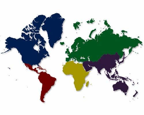
Map downloaded from: http://www.winrock.org/programs/images/world_map-2.jpg.
16Figure 3. Location of greenhouse gas emissions from a dairy farm in the UK: Case
study farm 1, a) system boundary 2, scenario 2, b) system boundary 2, scenario 3
a) Farm 1, system boundary 2, scenario 2
UK
72.3%
Russia
Europe 3.8%
4.8%
South
America
18.2%
b) Farm 1, system boundary 2, scenario 3
UK
64.3%
Russia
Europe 3.4%
4.3%
South
America
27.2%
The bars illustrate where greenhouse gas emissions related to the production of farm inputs and from
soil and livestock occur. Emissions in Russia are related to the production of nitrogen fertiliser,
emissions in South America are related to the cultivation of soya beans used in concentrate feed and
emissions from land use change.
Map downloaded from: http://www.winrock.org/programs/images/world_map-2.jpg.
17Figure 4. Location of greenhouse gas emissions from a dairy farm in the UK: Case
study farm 2, a) system boundary 1, scenario 1, b) system boundary 2, scenario 1
a) Farm 2, system boundary 1, scenario 1
UK
52.2%
Europe
19.9%
South
America
23.0%
b) Farm 2, system boundary 2, scenario 1
UK
87.6%
Europe
5.2%
South
America
6.0%
The bars illustrate where greenhouse gas emissions related to the production of farm inputs occur.
Emissions in South America relate to the cultivation of soya beans used in concentrate feed.
Map downloaded from: http://www.winrock.org/programs/images/world_map-2.jpg.
18Figure 5. Location of greenhouse gas emissions from a dairy farm in the UK: Case
study farm 2, a) system boundary 2, scenario 2, b) system boundary 2, scenario 3
a) Farm 2, system boundary 2, scenario 2
UK
74.5%
Europe
4.4%
South
America
20.0%
b) Farm 2, system boundary 2, scenario 3
UK
65.7%
Europe
3.9%
South
America
29.8%
The bars illustrate where greenhouse gas emissions related to the production of farm inputs and from
soil and livestock occur. Emissions in South America relate to the cultivation of soya beans used in
concentrate feed and emissions from land use change. Map downloaded from:
http://www.winrock.org/programs/images/world_map-2.jpg.
194. Discussion
Although the case study farms are different in terms of size and farming system
(conventional and organic conversion), they show very similar carbon footprints per
litre of milk. However, emissions per hectare are lower for case study farm 2 (in
organic conversion). As stated earlier, the footprint analysis does not allocate
emissions between different outputs from the farms, and therefore the estimated
carbon footprints presented here for milk are almost certainly an overestimate of the
real footprints. The footprint for the whole farm system, and for each hectare are
however accurate. Interesting as these footprint results are, the analysis of the
actual carbon footprint of milk is not the main purpose of this report, and these issues
will not be discussed further here (they will, however, be discussed in future
publications).
It is interesting to note that both farms show very similar carbon maps for their
emissions. When only considering the direct and embodied emissions from inputs it
is clear that less than 5 per cent of GHG emissions occur locally. Given the global
nature of the supply chains for major farm inputs, this pattern of emissions was
almost inevitable. When compared to other farm systems dairy farms tend to be
quite intensive users of inputs, however the main classes of inputs to all farm
systems are similar and include electricity, diesel, fertilisers and machinery. It is
therefore highly probable that similar carbon maps would be derived for all farm types
in the UK.
A complete analysis of the carbon footprints of food would not be restricted to
considering only direct inputs, as in system boundary 1. Rather, it would consider all
emissions from the farm system (as defined in system boundary 2). For dairy farms
this requires consideration of the methane emissions from enteric fermentation in
cattle and nitrous oxide emissions from livestock and soils. When these emissions
were included in the analysis they represented the greatest part of the carbon
footprint of both case study farms. Because these emissions occur directly on farm,
they were classed as truly local emissions, and as a result in all scenarios analysed
for system boundary 2, local emissions constituted more than 50 per cent of total
GHG emissions. Of course, as the GHGs ultimately disperse in the atmosphere their
impact is ultimately global. Indeed, it could be argued that as all GHG emissions
ultimately have a global impact, they have no relevance to the concept of local food.
However, this is not true for the stocks of carbon that are depleted during the
production of food and farm inputs. It is for this reason that the analysis considered
the production of soya for use in animal feed. This is an issue of particular concern
for animal production systems (including pigs and poultry), however it tends to
remain relatively poorly analysed as it is difficult to access information on the exact
nature of animal feed and the related levels of GHG emissions. Although some data
on the make up of dairy feed were obtained from formal and informal sources, these
data only enable rough estimates of the carbon footprint of animal feed, and they did
not explicitly include emissions related to any land use change which occurred in
order to enable production of the feed. For this reason it was necessary to develop
three specific scenarios for the production of soya: one assumed soya was produced
on land that had not previously been forested (scenario 1), and two scenarios
assumed savannah and/or forest clearance occurred in South America to enable
soya production (scenarios 2 and 3). In addition, the amount of soya in the animal
feed varied from an average of 16.5 per cent in scenario 2 to a maximum of 25 per
cent in scenario 3. As a result, the emissions from scenario 3 represent the worst
case situation for soya production. In this scenario 55 per cent of total emissions
20were classed as local for both case study farms, and as noted above over 95 per
cent of these would be related to the emission of methane from cattle and nitrous
oxide from soils.
This analysis raises several questions about the concept of local food in a globalised
market system. All UK farms derive inputs from outside the UK, and consequently
they are responsible for both the depletion of distant carbon stocks, and GHG
emissions that occur outside their locality. The concept of a carbon map offers a
method to represent the level of localness for any production system. The maps
presented here are very preliminary and tend to aggregate emissions at a large scale.
More detailed maps could be derived from closer analysis of relevant supply chains.
However, a detailed description of the supply chain would only provide part of the
map. A full analysis would also require detailed emission factors for the inputs and
their production processes. To date, much of the necessary data on both the supply
chains and the emissions are lacking, and further research would be needed in order
to operationalise the concept of the carbon map. If a carbon map could be
developed for different food types it would provide a means of visualising the impacts
of different food systems on the climate. Whether or not this information would be of
benefit to consumers, food chain professionals and/or policy makers remains
untested.
Further research
Further research is needed to develop this concept further in order to:
• develop more detailed analysis of supply chains and relevant emissions
factors (especially for livestock feed)
• obtain consumer feedback on the concept of the carbon map and document
perceptions of local and non-local emissions
• develop carbon maps for several different farming types, e.g. cereal,
vegetable, poultry. These may have different distributions for local and non-
local emissions as they would not include methane emissions from ruminant
livestock
• consider how the results of a carbon map could be included in regional
carbon accounts
• consider the variation in the carbon map between individual farms in a sector
• expand the analysis beyond the farm gate.
Conclusion
The data presented here pose serious questions about the validity of claiming that
any food is truly local. Less than 5 per cent of GHG emissions from the production
and use of inputs occur locally to the farm, and it is hard to conceive of a situation in
modern UK agriculture where this would not be the case. Emissions from livestock
and soils occur on farm, and are defined as local. Their inclusion in the analysis
increased local emissions to more than 55 per cent. Further analysis of the specific
emissions relating to the production of soya, which is a constituent of livestock feed,
identified the emissions from land use as being important constituents of the farms’
carbon footprints. Inclusion of these emissions in the analysis reduced the
21percentage of local emissions by up to 20 per cent. If UK farms want to localise
emissions then the most practical options are to:
• derive greater proportions of their energy needs from close by (e.g.
renewable or bioenergy)
• alter fertiliser strategy and seek substitutes for inputs of inorganic nitrogen
• reduce dependency on imported feed.
22References
Altieri, M. and Pengue, W. (2006). GM soybean: Latin America’s new coloniser. Seedling,
January 2006~: 13-17.
Bickel, U. and Dros, J.M. (2003). The impacts of soy cultivation on Brazilian ecosystems.
Three case studies. Report commissioned by the WWF Forest Conversion Initiative, available
at http://assets.panda.org/downloads/impactsofsoybean.pdf.
Brookes, G. (2001). The EU animal feed sector: protein ingredient use and implications of the
ban on use of meat and bonemeal. PG Economics. Available at:
http://www.pgeconomics.co.uk/pdf/mbmbanimpactjan2001.pdf.
Carbon Trust (2007). Carbon footprint measurement methodology. Version 1.3, 15 March
2007. see http://www.carbon-label.co.uk/pdf/methodology_full.pdf
Casey, J.W. and Holden, N.M. (2005). Analysis of greenhouse gas emissions from the
average Irish milk production system. Agricultural Systems 86: 97-114.
Casey, J.W. and Holden, N.M. (2006). Quantification of GHG emissions from suckler-beef
production in Ireland. Agricultural Systems 90: 79-98.
Castaldi, S., Costantini, M., Cenciarelli, P., Ciccioli, P., Valentini, R. (2007). The methane
sink associated to soils of natural and agricultural ecosystems in Italy. Chemosphere 66: 723-
729.
Chapuis-Lardy, L., Wrage, N., Metay, A., Chotte, J.-L., Bernoux, M. (2007). Soils, a sink for
N2O? A review. Global Change Biology 13: 1-17.
Charles, R., Jolliet, O., Gaillard, G., Pellet, D. (2006). Environmental analysis of intensity level
in wheat crop production using life cycle assessment. Agriculture, Ecosystems and
Environment 113: 216-225.
Cross, P., Edwards, R. T., Hounsome, B.,,Edwards-Jones, G. (2008). Comparative
assessment of migrant farm worker health in conventional and organic horticultural systems in
the United Kingdom. Science of the Total Environment 391: 55-65.
Dalgaard, R., Schmidt, J., Halberg, N., Christensen, P., Thrane, M., Pengue, W.A. (2008).
LCA of soybean meal. International Journal of Life Cycle Assessment 13: 240-254.
Defra (2006a). SCP evidence base: Sustainable commodities case studies. Case study Soya.
Department for Environment, Food and Rural Affairs, London.
Defra (2006b). EU emissions trading scheme – 2005 results for the UK. Summary sheet 7:
Lime sector. Department for Environment, Food and Rural Affairs, London, See
http://www.defra.gov.uk/environment/climatechange/trading/eu/ results/pdf/lime-summary.pdf
Department for Business, Enterprise & Regulatory Reform (2007). UK energy in brief July
2007. A National Statistics Publication.
Draper, A. and Green, J. (2002). Food safety and consumers: constructions of choice and
risk. Social Policy & Administration 36: 610-25.
Edwards-Jones, G., Milà i Canals, L., Hounsome, N., Truninger, M., Koerber, G., Hounsome,
B., Cross, P.A., York, E.H., Hospida, A., Plassmann, K., Harris, I.M., Edwards, R.T., Day,
G.A.S., Tomos, A.D., Cowell, S.J., Jones, D.L. (2008). Testing the assertion that ‘local food is
best’: the challenges of an evidence based approach. Trends in Food Science and
Technology 19: 265-274.
Ellingsen, H. and Aanondsen, S.A. (2006). Environmental impacts of wild caught cod and
farmed salmon – a comparison with chicken. International Journal of Life Cycle Assessment
11: 60-65.
Eriksson, I.S., Elmquist, H., Stern, S.,Nybrant, T. (2005). Environmental systems analysis of
pig production. International Journal of Life Cycle Assessment 10: 143-154.
23You can also read