Digital Commons @ Michigan Tech - Michigan Technological University

Michigan Technological University
 Digital Commons @ Michigan Tech

Dissertations, Master's Theses and Master's Reports

2016

Comparative Life Cycle Assessment of Road and Multimodal
Transportation Options - A Case Study of Copperwood Project
Sumanth Kalluri
Michigan Technological University, kalluri@mtu.edu

Copyright 2016 Sumanth Kalluri

Recommended Citation
Kalluri, Sumanth, "Comparative Life Cycle Assessment of Road and Multimodal Transportation Options - A
Case Study of Copperwood Project", Open Access Master's Report, Michigan Technological University,
2016.
https://doi.org/10.37099/mtu.dc.etdr/87

Follow this and additional works at: https://digitalcommons.mtu.edu/etdr

COMPARATIVE LIFE CYCLE ASSESSMENT OF ROAD AND
 MULTIMODAL TRANSPORTATION OPTIONS – A CASE
 STUDY OF COPPERWOOD PROJECT

 By
 Sumanth Kalluri

 A REPORT
 Submitted in partial fulfillment of the requirements for the degree of
 MASTER OF SCIENCE
 In Civil Engineering

 MICHIGAN TECHNOLOGICAL UNIVERSITY
 2016

 © 2016 Sumanth Kalluri

This report has been approved in partial fulfillment of the requirements for the Degree of MASTER
OF SCIENCE in Civil Engineering.

 Department of Civil and Environmental Engineering

 Report Advisor: Dr. Pasi T. Lautala

 Committee Member: Dr. David R. Shonnard

 Committee Member: Dr. William Sproule

 Committee Member: Dr. Robert M. Handler

 Department Chair: Dr. David Hand.

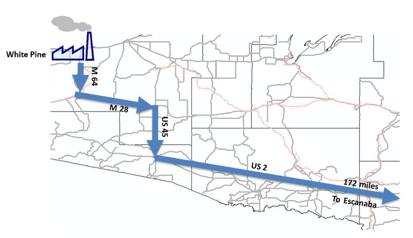
Table of Contents
Table of Contents ............................................................................................................................. i
List of Figures ................................................................................................................................ iv
List of Tables ................................................................................................................................. vi
Acknowledgements ....................................................................................................................... vii
Abstract ........................................................................................................................................ viii
Introduction ..................................................................................................................................... 1
 1.1 Background ...................................................................................................................... 1
 1.2 Study Objectives and Report Structure ............................................................................ 2
2 Life Cycle Assessment (LCA) ................................................................................................ 4
 2.1 Background ...................................................................................................................... 4
 2.2 LCA Phases ...................................................................................................................... 4
 2.2.1 Goal and Scope ......................................................................................................... 5
 2.2.2 Inventory Analysis .................................................................................................... 5
 2.2.3 Impact Assessment.................................................................................................... 5
 2.2.4 Interpretation ............................................................................................................. 5
 2.3 Life Cycle of a Product .................................................................................................... 6
 2.3.1 Construction/Manufacturing Stage ........................................................................... 6
 2.3.2 Use/Operations Stage ................................................................................................ 7
 2.3.3 End of Life ................................................................................................................ 7
 2.4 LCA in Transportation ..................................................................................................... 7
 2.5 LCA Databases and Software .......................................................................................... 8
 2.6 Impact Assessment Methods ............................................................................................ 9
3 Copperwood Project.............................................................................................................. 10
 3.1 Introduction .................................................................................................................... 10
 3.2 Ore Transportation Options ............................................................................................ 11
 3.2.2 Ore Transportation – Operational Characteristics .................................................. 16
 3.2.3 Ore Transportation – Maintenance ......................................................................... 17
 3.3 Concentrate Transportation Options .............................................................................. 18

 i

3.3.1 Alternatives of Concentrate Transportation ............................................................ 19
 3.3.2 Concentrate Transportation - Operation Characteristics......................................... 23
 3.3.3 Concentrate Transportation – Maintenance ............................................................ 24
4 LCA Application................................................................................................................... 25
 4.1 Goal and Scope of the Project: ....................................................................................... 25
 4.1.1 Functional Unit ....................................................................................................... 25
 4.1.2 System Boundary .................................................................................................... 25
 4.2 Inventory Analysis: ........................................................................................................ 25
 4.2.1 Manufacturing or Construction ............................................................................... 26
 4.2.2 Use/Operations ........................................................................................................ 35
 4.2.3 Maintenance ............................................................................................................ 38
 4.2.4 End of Life .............................................................................................................. 41
5 Results and Discussion ......................................................................................................... 42
 5.1 LCA Results for Primary Input Units ............................................................................ 42
 5.1.1 Construction/Manufacturing ................................................................................... 44
 5.1.2 Operations ............................................................................................................... 44
 5.1.3 Maintenance ............................................................................................................ 44
 5.2 LCA Results – Ore Transportation................................................................................. 44
 5.2.1 Ore Transportation – 20 Year Mine Life ................................................................ 44
 5.2.2 Ore Transportation – All Mine Lives...................................................................... 45
 5.2.3 Ore Transportation – Breakdown of Activities for 20 year Mine Life ................... 46
 5.3 LCA Results – Concentrate Transportation ................................................................... 47
 5.3.1 Concentrate Transportation – 20 Year Mine Life ................................................... 48
 5.3.2 Concentrate Transportation – All Mine Lives ........................................................ 49
 5.3.3 Concentrate Transportation – Breakdown of Activities for 20 Year Mine Life ..... 49
6 Integration of LCA into Economic Analysis ........................................................................ 51
 6.1 LCCA in Transportation................................................................................................. 52
 6.2 Methodology .................................................................................................................. 52
 6.3 Calculation of Costs ....................................................................................................... 53
 6.4 Integration of LCA into Economic Analysis.................................................................. 53
 6.5 Cost of Carbon ............................................................................................................... 54

 ii

6.6 Calculation of Emission costs ........................................................................................ 57
 6.7 Emission Cost Results .................................................................................................... 57
7 Conclusions and Recommendations for Future Research .................................................... 59
 7.1 Conclusions .................................................................................................................... 59
 7.2 Recommendations for Future Research ......................................................................... 60
References ..................................................................................................................................... 61
Appendix ....................................................................................................................................... 64
 Appendix -A: Inputs to SimaPro datasets ................................................................................. 64
 Appendix –B: Emission Cost Calculation ................................................................................ 71

 iii

List of Figures
Figure 1: Total U.S. Greenhouse gas emissions by economic sector in 2013 ................................ 1
Figure 2: Copperwood Mine and White Pine Processing Plant in Wester Upper Peninsula of
Michigan ......................................................................................................................................... 3
Figure 3: LCA Phases Outline (Source: ISO 14040) ...................................................................... 4
Figure 4: Stages of LCA – Cradle to Grave (Source: [10]) ............................................................ 6
Figure 5: Location Map of Copperwood, White Pine and Escanaba ............................................ 10
Figure 6: Movements Analyzed in the Study ............................................................................... 10
Figure 7: Ore Transportation, Location of Copperwood and White Pine (Road = Black, Track =
Red) ............................................................................................................................................... 11
Figure 8: Infrastructure and Route Comparison of Ore Transportation options between Mine and
White Pine..................................................................................................................................... 12
Figure 9: Ore Transportation Option A Road - Route Characteristics ......................................... 13
Figure 10: Ore Transportation Option B Multimodal (Road – 8 miles) - Route Characteristics . 14
Figure 11: Ore Transportation Option C Multimodal (Road – 3 miles) - Route Characteristics . 15
Figure 12: Concentrate Transportation, Location of White Pine and Mass City.......................... 18
Figure 13: Infrastructure and Route Comparison of Concentrate Transportation Options between
White Pine and Escanaba .............................................................................................................. 19
Figure 14: Concentrate Transportation Option D Road - Route Characteristics .......................... 20
Figure 15: Concentrate Transportation Option E Multimodal - Route Characteristics ................ 21
Figure 16: Concentrate Transportation Option F Multimodal - Route Characteristics ................ 22
Figure 17. LCA Process Outline ................................................................................................... 26
Figure 18: Screen shot of RTC Simulation including the Train Speed, Throttle, Braking and the
Track Elevation from Top to Bottom............................................................................................ 36
Figure 19 Global Warming Potential (GWP) of Different Ore Transport Options, for 20 years
Mine Life. ..................................................................................................................................... 45
Figure 20 kg of CO2eq per ton of Ore Transported in Different Options for all Mine Lives. ...... 46
Figure 21 Breakdown of GWP Emissions of Different Stages in Option B Ore Transport for 20
Years Mine Life ............................................................................................................................ 47

 iv

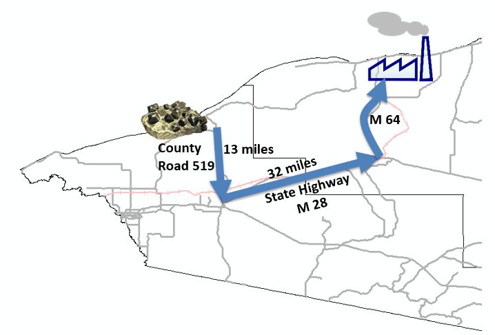
Figure 22 Global Warming Potential (GWP) of Different Concentrate Transport Options, for 20
years Mine Life. ............................................................................................................................ 48
Figure 23 kg of CO2eq per ton of Concentrate Transported in Different Options for All Mine Lives.
....................................................................................................................................................... 49
Figure 24 Breakdown of GWP Emissions of Different Stages in Option E Concentrate Transport
for 20 Years Mine Life ................................................................................................................. 50
Figure 25: Overview of Benefit Cost Analysis and Economic Impact Analysis (Source: [28]) .. 51
Figure 26 Integration of LCCA into LCA .................................................................................... 54
Figure 27: Calculation of Emission Costs .................................................................................... 57
Figure 28 Emission Costs per ton of Ore Transported ................................................................. 58
Figure 29 Emission Costs per Ton of Concentrate Transported ................................................... 58

 v

List of Tables
Table 1 Impact Assessment Methods in SimaPro........................................................................... 9
Table 2: Infrastructure Requirements for Ore Transportation ...................................................... 15
Table 3: Operational Data for Ore Transportation Options. ......................................................... 17
Table 4: Infrastructure Requirements for Concentrate Transportation ......................................... 22
Table 5: Operational Data for Concentrate Transportation .......................................................... 23
Table 6: Datasets of Processes under Infrastructure Construction ............................................... 27
Table 7 Hot Mix Asphalt (HMA) Custom Dataset – Quantities and Calculations ....................... 28
Table 8: Road Reconstruction (Heavy) Process – Quantities and Calculations per mile ............. 29
Table 9: Track Construction Process – Quantities and Calculations per mile .............................. 30
Table 10: Track Rehabilitation Process – Data and Calculations ................................................. 31
Table 11: Datasets for Processes under Rolling Stock Manufacturing......................................... 32
Table 12: Truck Manufacturing Process – Quantities and Calculations per Truck ...................... 33
Table 13: Loader Manufacturing Process – Quantities and Calculations ..................................... 34
Table 14: Locomotive and Rail Car Manufacturing Process - Quantities and Calculations per unit
....................................................................................................................................................... 35
Table 15: Ore Transportation – RTC Simulation Data ................................................................. 37
Table 16: Concentrate Transportation – RTC Simulation Data.................................................... 37
Table 17: Datasets of Processes under Infrastructure Maintenance ............................................. 38
Table 18: Track Maintenance Process– Quantities and Calculation per mile .............................. 39
Table 19: Datasets for Processes under Rolling Stock Maintenance ............................................ 39
Table 20: Truck Maintenance Process – Quantities and Calculations per mile ........................... 40
Table 21 Global Warming Potential in kg CO2eq per Unit for Primary Inputs ............................ 43
Table 22: Social Cost of Carbon Dioxide in 2014 dollars per metric ton CO2 (Source: EPA
Website) ........................................................................................................................................ 55
Table 23: Emissions breakdown of Option B (Ore Transportation) for 30 years Mine Life........ 56

 vi

Acknowledgements
 I would like to acknowledge the efforts given by my advisor, Dr. Pasi Lautala, without
whom the project was impossible for me to complete. He always encouraged me to come up with
new ideas and implement those in my project. He was always patient, supportive and helped me in
the technical and academic aspects of the project.
 I would like to thank my committee members, Dr. David Shonnard, Dr. William Sproule
Dr. Robert Handler, for their guidance and assistance in completing this report. Dr. Handler
provided me with valuable comments on my research from the beginning, which gave me the
direction I needed to undertake for my analysis. He spent a lot of time with me to provide
suggestions and improvements that were required for the LCA and also helped with the SimaPro
software.
 There are many people whom I would like to express my gratitude for assisting me in
completing my project. David Nelson provided me with valuable comments and suggestions to
improve this report. Hamed Pouryousef, provided assistance in performing the RTC simulation
runs to calculate the train fuel consumption. Aaron Dean also helped in developing the profiles for
the RTC simulation. Soumith Oduru provided assistance in analyzing the different LCCA tools
and summarizing them.
 I would like to thank Mr. Carlos Bertoni from Highland Copper and Mr. Tom Sullivan from
MHF Services for providing information about Copperwood project. Their guidance helped me to
gain knowledge about freight transportation and help. Mr. Darren Pionk, Gogebic County Road
Commission and Mr. Jim Iwanicki, Marquette County Road Commission provided the essential
data for road reconstruction and maintenance. Mr. Jim Delmont of M.J. VanDamme trucking for
assisting on the data related to trucking industry. Mr. Clint Jones and Mr. Christopher Jones
provided guidance on the data related to track construction, track maintenance and locomotive
maintenance.
 This research was supported by National University Rail (NURail) Center, a US DOT-
ST Tier 1 University Transportation Center and the Michigan Department of Transportation

 vii

Abstract

Freight transportation of goods and commodities is a necessity and often accounts for a significant
portion of the overall investment in the industrial development, especially in the natural resource
industry. The economic costs of developing an infrastructure have long been factored into the
project costs, but environmental and/or social impacts have received less attention. In addition,
alternative transportation modes are rarely compared from both economic and environmental
perspectives. This project uses a case study to assess the environmental impacts (emissions) of
different transportation options for transporting ore between a planned mine and a processing
plant, and concentrate from the processing plant to an intermediate location (Escanaba, MI). The
ore transportation options include truck only option and two multimodal (truck-rail) options, while
the concentrate transportation options include truck only, rail only and one multimodal (truck-rail)
option.
Environmental impact assessment is done by a process called Life Cycle Assessment (LCA) using
SimaPro Version 8 software and includes all aspects related to the construction, operation, and
maintenance (stages) of transportation infrastructure and equipment required for the project. The
end of life stage was excluded from the analysis. The different processes that occur during the
three stages are identified and data for each process is either collected from local sources or from
datasets available in SimaPro. The analysis is conducted for four alternative mine lives, ranging
from ten to thirty years.
The output of the LCA is provided in the overall Global Warming Potential (GWP) in terms of
kilogram equivalents of CO2 (kg CO2eq) and the emissions generated by each transportation option
are compared on the basis of one ton (US ton) of ore/concentrate transported. Overall, the results
suggest that multimodal options generate the lowest emissions among all alternatives, for both ore
and concentrate transportation. Operations stage accounts for the majority of the emissions for all
six options, regardless of the life of the mine, but there are large differences in the operational
emission quantities from truck only vs. multimodal options. It is also revealed that the construction
emissions can be significant, especially for short mine lives, but emissions from maintenance
activities remain fairly low for all options and all mine lives.
In addition to quantifying the emissions from each alternative, the integration of results into
economic analysis is investigated. An overview of Life Cycle Cost Analysis (LCCA) for freight
transportation options is discussed and the emission results from LCA are converted to dollar value
for transporting one ton of ore/concentrate using costs of carbon from literature.

 viii

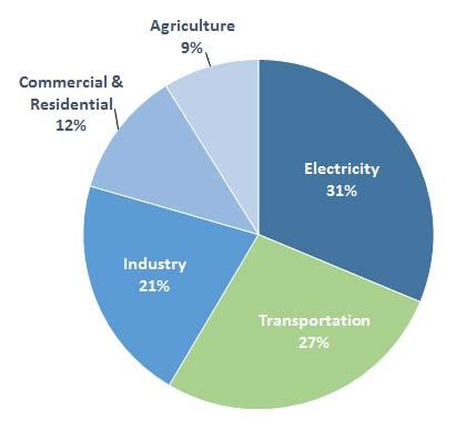
Introduction
1.1 Background
 Freight transportation commonly occurs between the major steps of a production system
and is very important in a product’s life cycle. Energy consumed by the transportation sector is
one of the major sources of emissions and tailpipe emissions from transportation accounted for
27% of the total greenhouse gas (GHG) emissions in the United States (US) in 2013 (Figure 1).
Almost one quarter (23%) of these emissions were from the medium and heavy duty vehicles [1]
and forecasts indicate that the fuel consumption by heavy duty vehicles will increase by 25% from
2013 to 2040, even though the consumption of light duty vehicles is currently declining [2].

 Figure 1: Total U.S. Greenhouse gas emissions by economic sector in 2013
 (Source: United States Environmental Protection Agency. Sources of Greenhouse Gas Emissions:
 Transportation Sector Emissions[1])

 Due to the forecast of an increase in heavy duty vehicle emissions, it is essential that new
freight transportation projects take up measures to minimize fuel consumption/emissions
throughout the project life cycle. To initiate the process, in June 2015 the EPA proposed a phase
two rulemaking process for reduction of greenhouse gas emissions and fuel consumption standards
of medium and heavy duty engines and vehicles. The EPA also published Tier 4 emission standards
in 2008 to control the emissions from off road vehicles and locomotives built after 2015 [3]. These
standards regulate the emissions from idling locomotives and target the reduction of particulate
matter (PM) by as much as 90% and the NOx emissions by 80 % [4]. With these regulations in
place, the CO2 emissions and fuel consumption of heavy duty vehicles would decrease by 24% of
the current values, instead of the increases predicted above [5].

 1

While operational (tailpipe) emissions are well understood and accounted for, the
construction and maintenance activities of roads, railroad tracks, and various other transport
infrastructure are also significant contributors to project level emissions. To minimize the overall
impacts of a project to the environment, it is essential that all contributing activities throughout the
project life cycle be considered. To secure this, quantification and comparison of emissions
between different project alternatives should be a standard procedure during the development. This
is commonly done to compare the economic attributes of roads/highways to determine the
preferred project alternatives for developing new infrastructure [6]. It may also be done for cases
where different modal alternatives can be considered (such as rail versus road), but detailed
environmental (emissions) comparison between those alternatives have rarely been conducted.
Life Cycle Analysis (LCA) looks at the overall environmental impacts and emissions released by
a product or project over its life time.

1.2 Study Objectives and Report Structure
The objective of the study was to use a process called Life Cycle Assessment (LCA) to conduct
environmental impact assessment for different transportation alternatives considered for the
Copperwood Project, a planned copper mine and processing plant in the Upper Peninsula of
Michigan (Figure 2). The study will investigate transportation alternatives for both ore and
concentrate transportation movements and will consider four different mine lives for the analysis.
Specific objectives of the study are
 • Review the concept of LCA and past literature on its applications in transportation
 projects. This includes reviewing past studies on transportation infrastructure
 construction, maintenance and operations, and those related to equipment
 construction maintenance and operations.
 • Perform impact assessment for the ore and concentrate transportation options of
 the Copperwood project.
 o Identify, develop and collect necessary parameters and related data for each
 option
 o Interpret and summarize the LCA emission results of alternatives.
 • Investigate the economic methodologies for analyzing transportation system
 investments and integration of LCA results into the analysis.
 • Perform conversion of emissions to dollar values using available costs of carbon.

 2

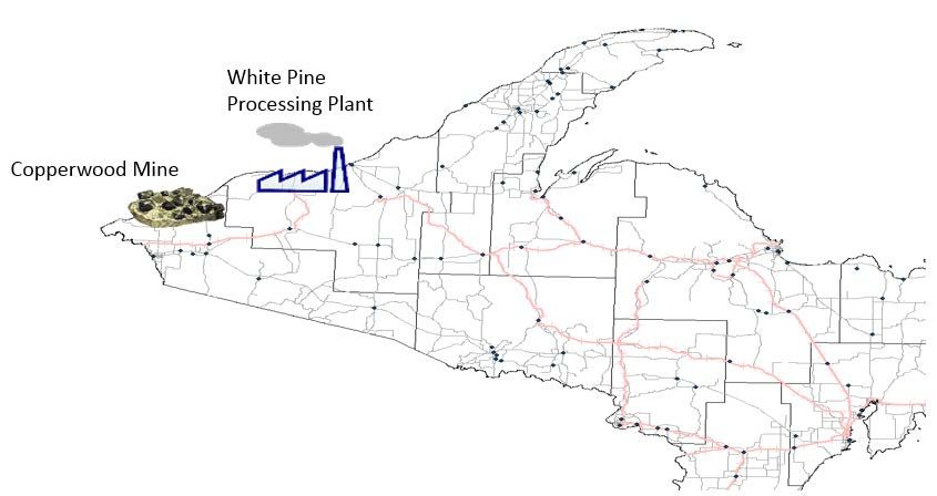
Figure 2: Copperwood Mine and White Pine Processing Plant in Wester Upper Peninsula of Michigan
 The report is broken down to seven chapters. Chapter two will start by defining LCA and
reviewing its past applications in transportation projects. We also discuss a brief outline of the
LCA process in this chapter. Chapter three introduces the case study and related transportation
alternatives investigated in the project and in Chapter four we review the data and tool for the LCA
analysis. In Chapter five, the results for the LCA are provided and discussed in detail. The current
methodologies for transportation investment decision making and the integration of emission
results into overall decision making by converting them to costs is discussed in Chapter six. The
final chapter includes project conclusions and next research steps.

 3

2 Life Cycle Assessment (LCA)
2.1 Background
 Life Cycle Assessment (LCA) is a method of assessing environmental impacts over a
product or process life cycle, ideally from raw material extraction to the final end of life stage. The
demand for sustainable products has encouraged the development of LCA in order to quantify
potential impacts of product changes. The history of LCA dates back to 1969 when Coca-Cola
first conducted a LCA study to compare the impact of different beverage container materials on
the environment [7]. Since then LCA became a commonly used process and several technical
societies established guidelines and standards for conducting an LCA. In 1993, the International
Organization for Standardization (ISO) began the standardization of the LCA process. The
outcome was the initial Principles and Frameworks of LCA – ISO 14040 in 1997 [8] and the
framework defined a method for performing a simple LCA process and listed all the terms and
principles. Numerous revisions were made to these guidelines before the final ISO 14040 – LCA
Requirements and Guidelines was compiled in 2006 [9]. This framework described more elaborate
methodology to perform LCA for a product or a process.

2.2 LCA Phases
 The phases of LCA outlined by ISO 14040:2006 [9] include all the processes and
methodology to perform LCA for a typical product life cycle. According to the outline, LCA is
performed in four different phases: Goal and Scope Definition, Inventory Analysis, Impact
Assessment, and Interpretation. Figure 3 shows a general outline of LCA phases.

 Goal and
 Scope
 Definition

 Inventory
 Interpretation
 Analysis

 Impact
 Assessment

 Figure 3: LCA Phases Outline (Source: ISO 14040)

 4

2.2.1 Goal and Scope
 In this phase the primary goal of the LCA is identified, and the functional unit and
boundaries for performing LCA are set. The functional unit can be used as a reference to compare
two or more competing methods or systems. Boundary definition includes identifying the stages
of the product life cycle included in the LCA. All the processes that are included and excluded
from the LCA are defined in the boundary. For example, if there are any repetitive processes when
performing comparative LCA of two products, we can define in the boundary if we want to include
or exclude the repetitive process. Also the time frame for LCA and the environmental impacts to
be assessed are defined in this phase.
2.2.2 Inventory Analysis
 Identifying the inputs to the processes that occur during the life cycle of a product is done
in the inventory analysis phase. This includes defining all of the primary material and energy inputs
of a process based on the defined boundary, as well as the secondary inputs of energy, material
and transport processes that are required for all the primary inputs. The data for the secondary
inputs is typically included in the lifecycle inventory databases. If the data for any of the primary
or secondary inputs does not meet the required process or flow, then custom datasets are created
in the databases by collecting the necessary information of the process. All material data and
custom databases are validated with the help of different existing databases and scientific values.
2.2.3 Impact Assessment
 In an impact assessment, the method for analysis is selected to produce the desired output
of the LCA. Methods can include calculating the total energy consumed over the life of a product,
calculation of total resource consumption over the product life cycle, calculating the total
greenhouse gas emissions in terms of CO2 equivalents, quantifying human health impacts and
resource consumption among many other methods available. They are often developed by a team
of researchers after careful study of the relevant literature; and are updated as necessary, to reflect
new information of life cycle inputs and related environmental impacts. A more detailed discussion
on different impact assessment methods is presented in section 2.6.
2.2.4 Interpretation
 In this phase, impact assessment results are analyzed based on the desired output of the
LCA. Sensitivity analysis and uncertainty analysis for the parameters are also done in this phase.
Based on the outcomes, recommendations can be made to revise the data inputs and/or the system
boundary to perform the LCA iteratively. The results of the iteratively performed LCA can be used
to compare alternatives with different input values and also help identify the processes with most
impacts in the life cycle of the product.

 5

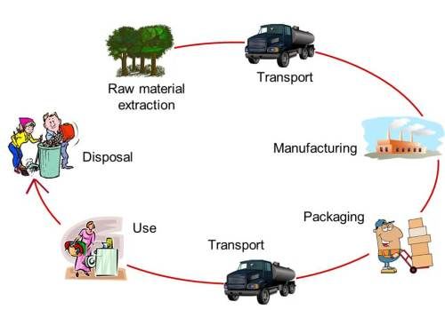
2.3 Life Cycle of a Product
 Since all of the processes that release emissions into the environment during the life of a
product are measured, LCA is considered a “cradle to grave analysis”. The basic stages of a life
cycle are manufacturing/construction of the product (including gathering of raw materials),
use/consumption, and finally the end of life stage which include the products disposal and return
of materials to earth. The different processes under each stage are categorized separately before
performing LCA, so that the amount of emissions or environmental impact from each process of
the product’s life cycle can be identified. Figure 4 shows an example of different stages and the
processes that occur in the life cycle of a product, followed by discussion of each key stage to our
case study.

 Figure 4: Stages of LCA – Cradle to Grave (Source: [10])

2.3.1 Construction/Manufacturing Stage
 The processes that are undertaken to develop, construct or manufacture a product are part
of the construction/manufacturing stage of an LCA. This includes the use of required resources
like raw materials, intermediate and / or finished products. The input data also includes the energy
consumption, the transport of the materials and other secondary level processes involved in the
construction. For example, the construction, or manufacturing stage of a light bulb includes the
glass production, energy consumed for the production of glass and other materials, transport of the
materials and the process for forming the shape of the bulb along with packaging. Here the primary
processes are glass production and packaging. The secondary level processes are energy consumed
for production of glass, transport to the market and packaging cardboard manufacturing process.

 6

2.3.2 Use/Operations Stage
 This includes all the processes that are involved during the use of the product, or operation
or maintenance of the product. Commonly, operations and maintenance of the product are all part
of the operations stage. As an example, for a light bulb’s LCA, the use/operations stage includes
the consumption of electricity and the production of this electricity. However, for our case study,
we considered the operations stage and maintenance stage separately, as we wanted to be able to
quantify the operations vs. maintenance born emissions in more detail.
2.3.3 End of Life
 The end of life stage of the LCA includes the different materials that are disposed of or
recycled after the use of the product or a process. Considering the same example of the light bulb,
the end of life includes the disposal and/or recycling of the glass and metal components of the
bulb. End of life was excluded from our case study analysis, due to the uncertainty of actions at
the end of project.

2.4 LCA in Transportation
 Use of life cycle assessment in the transportation sector has gained prominence during the
last decade and the development of reliable datasets and guidelines has enhanced its capabilities
to explore the impacts of transportation on the environment. The earlier datasets and LCA methods
included the impacts caused by transport of goods, raw materials and other processed materials
over an average distance, but considered only the tail pipe emissions of the transport process. The
study by Facanha and Horvath was one of the few to include all the infrastructure, vehicle and fuel
life cycle phases [11]. LCA analysis on complete highway freight transport project was first
performed in Germany by Marheineke in a study which included the production, use, and end of
life for trucks, along with related road construction and maintenance.
 LCA is typically performed using process flow analysis, but Marheineke also used a hybrid
model of Input-Output analysis [12]. Spielmann used European data to develop a similar life cycle
inventory for the transport of goods by road, rail, and water [13]. His inventory is considered to be
one of the few which include complete life cycle stages of infrastructure, vehicles and fuel on
multiple modes [11]. Based on Spielmann’s approach, Facanha and Horvath tried to develop an
inventory with US data that can calculate the emissions of all the processes in transportation,
including the fuel life cycle, infrastructure provision, production and end of life of the rolling stock
[11]. The comparison of their LCA results with that performed for only tail pipe emissions indicate
that life cycles of vehicles and transportation infrastructure account for a significant amount of
total emissions. Argonne National Laboratory in the US has been conducting several studies on
the life cycle analysis of long distance freight transport over land. One of them highlighted the
emissions during the manufacturing of vehicles and extraction and combustion of fuels during the
freight transport process of a vehicle. It also compared the emissions from alternative fuels over
the life cycle [14]. In the early 2000’s, Argonne developed the Greenhouse gases, Regulated
Emissions, and Energy use in Transport (GREET) model as a tool for estimating the greenhouse

 7

gas emissions from the transportation life cycle, including fuel and vehicle stages. This model is
currently applicable to passenger cars and light duty truck life cycles only [15].
 The previous studies on the LCA process for road, trucks, railroad tracks, locomotives and
rail cars mostly discuss all off the data inputs necessary to conduct LCA for the equipment (trucks
and rail rolling stock), but the data requirements for conducting infrastructure LCA have not been
detailed in any comparative study. Past studies that apply the LCA for road infrastructure exist,
but the boundaries and conditions differ from case to case [16]. For example, a study on pavement
construction scenarios included the different materials for construction of pavement, but
considered the construction equipment emissions static between cases [17]. LCA analysis on rail
infrastructure had similar differences in system boundaries and most of them relate to passenger
train infrastructure, partially due to their origination in Europe [18, 19]. A study by the New
Zealand transport agency on the lifetime liabilities of road and rail infrastructure attempted to
enhance the understanding of the emissions over the life of the infrastructures, but it only
considered the construction stage of the infrastructure and limited maintenance aspects while
neglecting the end of life considerations and maintenance of other critical parts [20].
 Modal comparisons are difficult to find in literature. A study by Kim [21] looked at
emissions between truck only and truck-rail intermodal systems in Europe. The study initially
identified that truck and rail based systems are not directly comparable due to the door to door
service provided by the trucks. A conceptual model was created in which the rail based intermodal
and truck only system offered similar service levels. From the results it was found that the
emissions from the rail based intermodal system were lower than from the truck only system, but
the proportion changed depending on the source of energy for the trains.
 The LCA of trucks and railroad rolling stock (trains) over their life cycle in freight
transportation are not as complicated as the infrastructure LCA and the procedures and inventories
are outlined to some extent in the past studies [11, 22, 23]. These inventories include all the stages
of construction, maintenance and the fuel use and emissions during their life. They are used as a
basis for the equipment life cycle inventory developed for this study.

2.5 LCA Databases and Software
 Analyzing the life cycle of a product involves various steps and processes that occur during
its useful life. Databases of the common products and their major life cycle processes have been
developed over the years to help perform the LCA. These databases are frequently provided with
updates, as scientific agencies and technical societies continue their development. A few
commonly used databases are the ecoinvent, US Life Cycle Inventory, and GaBi database
developed for GaBi tool. LCA tools and software integrate these databases with a user interface
for performing the LCA.
 SimaPro, OpenLCA, GaBi, Umberto and the GREET model are major tools for performing
LCA. The tools mainly differ in the type of interface and the impact assessment methods available;
and may only allow use of some of the databases listed above. The GREET model is mostly used

 8

for transport related LCA and includes LCA of fuels and related transport processes. The tool
calculates the emissions, as well as other criteria pollutants that result from transportation life
cycles. OpenLCA is an open source software platform that primarily uses the ecoinvent and GaBi
tool databases. The software is run and managed by the Green Delta company of Germany, and
can be downloaded from their website.
 SimaPro 8.0 software was used to perform the LCA in this study. SimaPro is a European
software that relies on European databases. The main database is the ecoinvent v3.1 that has more
than 10,000 processes and flows in areas like chemicals, agriculture, transport, and metals. It is
one of the most extensive databases in the world [24]. SimaPro also includes the US Life Cycle
Inventory database (USLCI) and the U.S. ecoinvent database is currently being added into the
software.

2.6 Impact Assessment Methods
 As described earlier, the output of LCA is determined based on the impact assessment
method selected for the analysis. Table 1 shows the three impact assessment methods available in
SimaPro.
Table 1 Impact Assessment Methods in SimaPro
 Method Output
 Total process and embodied energy required
 Cumulative Energy Demand
 in kJ or BTU
 Impacts of different pollutants and resource
 Eco Indicator 95 Method
 consumption.
 IPCC 2013 GWP 100a kg CO2 eq. of all the greenhouse gases.

 The IPCC 2013 GWP 100a method was used to quantify the equivalent amount of CO2
released over the life of the process. The global warming potential (GWP) of the different
greenhouse gas emissions released during the life cycle of a product are calculated in this method.
All non-carbon dioxide gas emissions are converted to equivalents of CO2 emissions and the final
output will be in equivalents of carbon dioxide (kg CO2 eq.). In GWP, the potential of a gas or
atmospheric pollutant is calculated for 20, 100, and 500 year time intervals. GWP of a gas is
defined as the ability to absorb energy from the earth that would otherwise escape into space,
resulting in heating up of the atmosphere. The gases that can be quickly removed from the
atmosphere will have a higher potential over short time horizons and lower potential over longer
time horizons. The 100a indicates a 100 year time period over which the potential of a particular
gas is calculated. Since all the greenhouse gas emissions can be quantified in terms of CO2
equivalents, the IPCC method was selected for the analysis in this project.

 9

3 Copperwood Project
3.1 Introduction
 Highland Copper is a Canadian firm focused on exploring and developing copper mining
projects in the Western Upper Peninsula (U.P.) of Michigan Figure 5 [25]. In 2014 the company
acquired the copper deposits of Copperwood, White Pine North and Keweenaw “projects” and it
has completed the feasibility studies for potential copper ore mining at each project location, and
for the development of a processing facility at White Pine to convert the ore to copper concentrate.

 Figure 5: Location Map of Copperwood, White Pine and Escanaba
 It is estimated that about 2.7 million tons of ore will be produced annually (7,000 tons per
day) at the Copperwood mine site that is located in Gogebic County, approximately 20 miles west
of the White Pine (as the crow flies). The ore is then transported to the processing plant in White
Pine where it is converted to concentrate. The quantity of concentrate produced after processing is
10% of the ore volume, or approximately 270,000 tons annually. The remaining 90% of the ore
(tailings) will be placed in the existing tailings pond near the processing plant. The concentrate is
transported from White Pine to a currently unidentified location for further processing. It is
expected that the concentrate transportation will travel through Escanaba, which is a regional
transportation hub with good ship and rail connectivity Figure 6.

 Location: Location: Transport Location :
 Transport
 Copperwood White Pine Concentrate Escanaba
 Ore to
 to
 Activity: Processing Activity: End of
 Intermediate
 Mine Ore Plant Process Ore Study
 point

 Figure 6: Movements Analyzed in the Study

 10

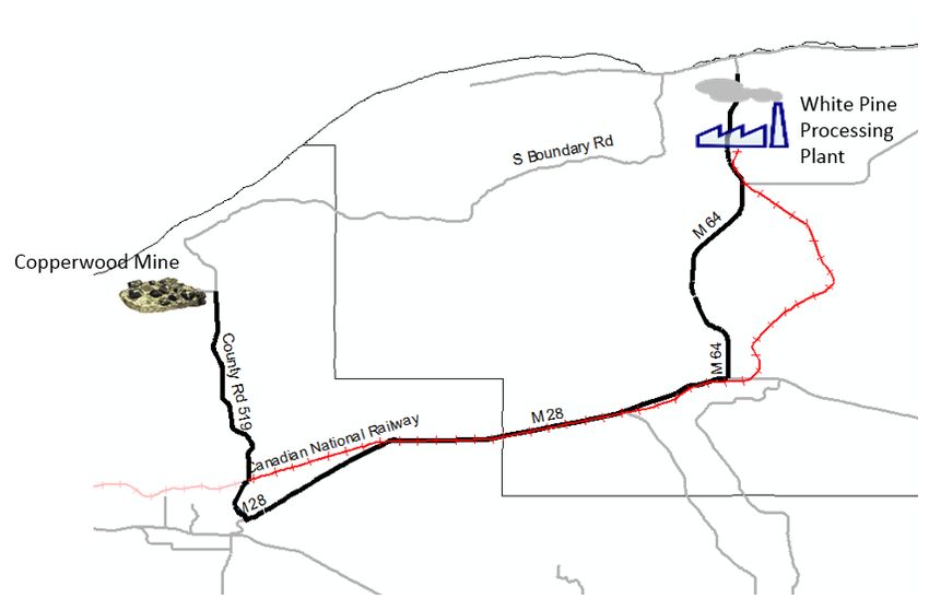
Since the final destination for concentrate has no effect on the ore transportation decisions
from the mine to White Pine and on the concentrate transportation from White Pine to Escanaba,
this study concentrates on evaluating the alternatives for those two movements Figure 5. After
Escanaba, Highland Copper will have the choice of selecting the most economic mode available
for the final leg of concentrate transportation.
 The different options for transporting ore and concentrate are discussed in following
sections. For all options, the overall environmental effects will be evaluated using LCA tools and
from the results of the LCA, a preferred option for the transportation of ore and concentrate from
environmental perspective will be identified.

3.2 Ore Transportation Options
 As mentioned above, the ore mined in Copperwood is to be transported to the
processing plant in White Pine (Figure 7). As the Copperwood site is only two miles from the
South Boundary Road of the Porcupine Mountain state park, specific consideration is placed in
avoiding the use of that road and thus minimizing the effects of the project on park activities.

 Figure 7: Ore Transportation, Location of Copperwood and White Pine (Road = Black, Track = Red)

 11

Highland Copper is looking at three alternative routes that partially rely on existing road
and rail infrastructure, and use either single or multimodal transportation. The options are shown
in Figure 8 and discussed in the following sections.

 Figure 8: Infrastructure and Route Comparison of Ore Transportation options between Mine and
 White Pine

3.2.1.1 Option A: Road Transportation
 In this option, the ore is transported from the mine to the processing plant by trucks. The
route for this option travels south from the mine for 13 miles on County Road 519 until the road
meets M 28, follows M 28 east 19 miles and turns north at Bergland onto M 64 for 13 miles until
reaching the processing plant in White Pine. (Figure 9). The state highways are currently all season
roads capable of handling the ore trucks, but the county road must be upgraded to facilitate the
24/7 movement of trucks throughout the year. County road upgrade includes heavy reconstruction
of the full 13 miles. The total length of one way road trip from the mine to White Pine in Option
A is 45 miles.

 12

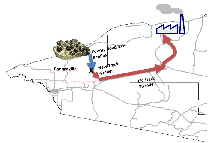
Figure 9: Ore Transportation Option A Road - Route Characteristics

3.2.1.2 Option B: Multimodal Transportation (Road – 8 miles)
 This is a multimodal option in which the first 8 miles from the mine to Connorville location
is by truck on County Road 519. A transload facility will be constructed at Connorville and the
ore will then be transported 34 miles by train to White Pine in hopper style rail cars. The county
road in this option has to be reconstructed heavily for full 13 miles. For the rail movements, there
is an existing CN railway line from Thomaston to White Pine, which hasn’t been used since 2010,
and requires rehabilitation of track structure and the subgrade. The track from Connorville to the
existing CN line must be constructed on an old track subgrade. For Option B, the length of road
trip is 8 miles, followed by 34 miles for one way train movement (Figure 10).

 13

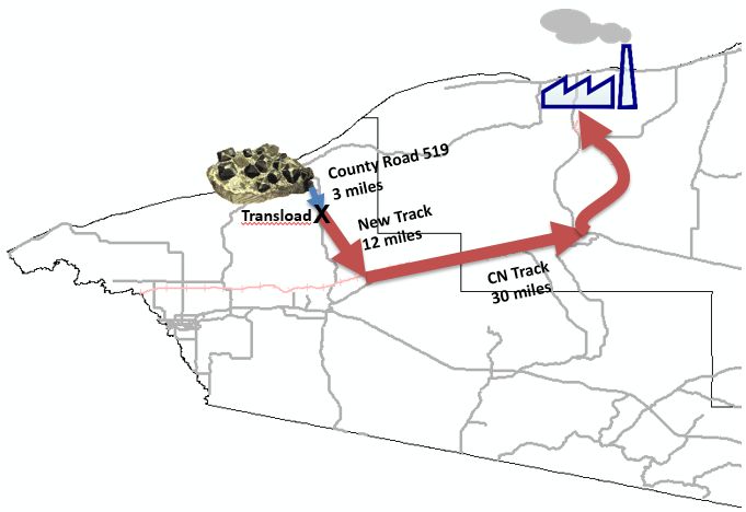
Figure 10: Ore Transportation Option B Multimodal (Road – 8 miles) - Route Characteristics

3.2.1.3 Option C: Multimodal Transportation (Road – 3 miles)
 The third option is also a multimodal option in which the ore will be trucked for the first
three miles and then it is transloaded into hopper cars and transported by train 42 miles to White
Pine. First three miles must be trucked due to high grades and land constraints which make it very
expensive to build new track all the way to the mine. In the analysis, three miles of heavy
reconstruction was considered for the county road, while the remaining 10 miles requires light
upgrade for service vehicles. However, per Highland Copper, it is plausible that heavy
reconstruction is required for the full 13 miles. The rail route from the transload facility to the
existing CN track follows an old track and requires 12 miles of new track construction on existing
subgrade. Rehabilitation (same as Option B) is required for the existing CN track. A transload
facility must be constructed three miles south of the mine to load the rail cars. In this option, the
length of one way truck trip is three miles and length of train transport is 42 miles (Figure 11).

 14

Figure 11: Ore Transportation Option C Multimodal (Road – 3 miles) - Route Characteristics
 Table 2 shows the comparison of infrastructure requirements for each ore transportation
option.
Table 2: Infrastructure Requirements for Ore Transportation
 Option A Option B Option C

 Transport by Road (miles) 45 8 3

 Transport by Rail (miles) N/A 34 42
 Road Heavy
 13 13 3
 Reconstruction miles
 Light Road Upgrade miles 0 0 10
 New Track Construction
 on Existing Track Bed N/A 4 12
 (miles)
 Track Upgrade (miles) N/A 30 30

 Transload construction No Yes Yes

 15

3.2.2 Ore Transportation – Operational Characteristics
 The data for truck and rail equipment and operations was provided by Highland Copper,
MHF services (project consultant for Highland Copper), and M.J. VanDamme trucking. The trucks
used for the ore transport are Michigan 11-axle tractor-trailer trucks with a gross weight of 164,000
lbs. (82 tons). They have a carrying capacity of 51 tons, and will be operated 24/7 throughout the
year. 140 round trips are required per day. Due to confidentiality, the total number of trucks is not
disclosed in the report.
 Snow on the county road 519 must be cleared during winter, so that the operations are not
interrupted. Since the snow clearing requirements on the county road must be expanded due to the
opening of the mine, the operation of snow plows will have impact on the overall emissions of ore
transport. The snow clearing for the 13 miles of county road will be accounted for in the analysis.
 The rail cars used for the ore transport are covered hoppers of net capacity 100 tons per
car. 70 rail car loads of ore have to be transported daily from the mine to the processing plant. Two
2,000 horsepower locomotives will be used to haul the trains. The train operation for Option B is
one train trip per day, but in Option C, two 35 car trains will be operated from transload near the
mine to Connorville where they are combined into one 70 car train to White Pine. This is due to
the steep ascent from the mine to the existing CN track that makes two locomotives insufficient
for hauling 70 cars at once. In the return, all the 70 cars can be pulled back to the mine transload
location.
 The rail cars will be loaded at the transload facility using one front end loader. The
transload building will be covered and the trucks use side dumps to unload the ore. Table 3 gives
a detailed outline of the operational characteristics of ore transportation.

 16

Table 3: Operational Data for Ore Transportation Options.
 Option A Option B Option C
 Annual tons of ore 2.7 million
 Net Capacity of
 51 tons
 trucks
 Total number of
 XX YY ZZ
 trucks
 Truck round trip
 90 16 6
 (miles)
 Train round trip
 N/A 68 84
 (miles)
 Number of truck
 140
 trips per day
 Number of
 N/A 2 – 2000 HP 2 – 2000 HP
 locomotives
 Total number of
 N/A 70 70
 rail cars
 Gross(Net) weight of
 130(100) tons
 rail cars
 Cars per train trip N/A 70 35*
 Train roundtrips per
 N/A 1 2*
 day
 Transloading
 N/A Front End Loader
 Equipment
N/A - Not Applicable, XX - No. of trucks in Option A, YY - No. of trucks in Option B, ZZ - No. of trucks in Option C
* - In option C, two train trips per day from Mine to Connorville, From Connorville to White Pine it is one train.

3.2.3 Ore Transportation – Maintenance
 The maintenance of infrastructure and equipment is one of the most important tasks to keep
the project running without delays. The major maintenance of road is milling and overlay of the
13 miles of county road in five year intervals. State highway maintenance is excluded, as no change
is considered due to mine opening. The track maintenance includes annual inspections and spot
repairs. It was assumed that about 20% of the quantities of track construction are required for track
maintenance every five years. Also this maintenance is spread across the five year interval with
1/5th every year.
 Per MJ VanDamme, the preventive maintenance for trucks is done every 15,000 miles of
operations and includes change of hydraulic fluids, engine oil and lubricants. The drive and steer
tires have a life of 70,000-80,000 miles and the trailer tires have a life of 130,000 miles. Per

 17

Mineral Range Railroad, the locomotive and rail car maintenance includes the change of
lubricants, oil and rail car wheels periodically to keep the equipment in good condition. In the
analysis, the maintenance of locomotive includes the change of oils and filters once every month
and the rail car maintenance includes a wheel change every 300,000 miles of operations.

3.3 Concentrate Transportation Options
 The ore is received at White Pine and processed into higher value copper concentrate. The
concentrate will then be transported from White Pine to an as yet to be determined location. Since
all routes for concentrate transportation are expected to move through Escanaba, it was selected as
the end point of the study. The general route options for concentrate transportation are shown in
Figure 12.

 Figure 12: Concentrate Transportation, Location of White Pine and Mass City
 Just like for ore transportation, the Highland Copper is considering three alternatives for
the concentrate transportation between White Pine and Escanaba. These options are shown in
Figure 13 and discussed in the following sections.

 18

Figure 13: Infrastructure and Route Comparison of Concentrate Transportation Options between White
 Pine and Escanaba

3.3.1 Alternatives of Concentrate Transportation
3.3.1.1 Option D: Road Transportation
 In this option, the concentrate is transported from the processing plant to Escanaba by road.
The route follows along M 64 south from White Pine to Bergland for 13 miles, turns south to US
45 south for 19 miles from Bergland to Watersmeet and then follows US 2 east until Escanaba for
140 miles. Since most of the route is existing state highways, there is no need for new road
construction or major upgrades and no additional maintenance expenses are considered due to
concentrate traffic. The total length of one way trip from the White Pine to Escanaba is 172 miles
(Figure 14).

 19

Figure 14: Concentrate Transportation Option D Road - Route Characteristics

3.3.1.2 Option E: Multimodal Transportation
 This is a multimodal transportation option where trucks move concentrate from the White
Pine processing plant to transload facility in Mass City (33 miles). From Mass City the concentrate
will be transported 160 miles to Escanaba by train in covered hoppers. The infrastructure
construction and improvements for the road part of the transport are minimal, as this route uses
mostly state highways M 64, M 38 and M 26 which are in good condition. There might be a few
minor upgrades to the bridges and grade crossings, as necessary. Rail portion uses existing E&LS
railway line from Rockland to Escanaba, which passes through Mass City. This line is operational
and doesn’t require major upgrades. Initially the plan was to setup a transload facility at Rockland,
which is further west of Mass City, but due to short rail sidings and land availability issues, the
transload location was moved to Mass City. At Mass City, there are existing sidings which can be
upgraded and used for transloading, but better infrastructure for concentrate storage and handling
must be constructed. The length of one way road trip is 33 miles and one way train movement is
160 miles (Figure 15).

 20