A PARALLEL MONTE CARLO IMPLEMENTATION ON THE CELL BROADBAND ENGINE - MARCUS LUNDBERG - DIVA
←
→
Page content transcription
If your browser does not render page correctly, please read the page content below
IT 09 029

                                Examensarbete 30 hp
                                          Juni 2009

A Parallel Monte Carlo Implementation
on the Cell Broadband Engine

Marcus Lundberg

            Institutionen för informationsteknologi
               Department of Information Technology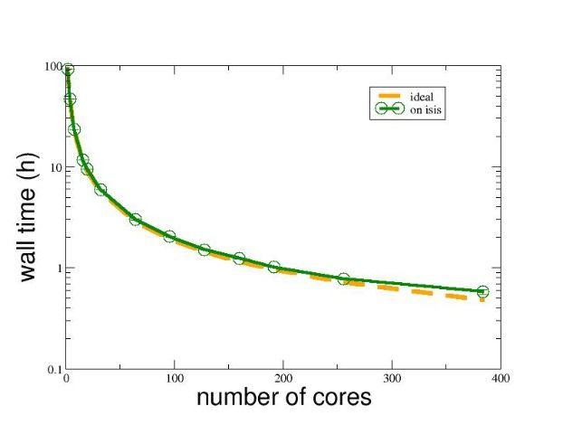
Abstract
                                      A Parallel Monte Carlo Implementation on the Cell
                                      Broadband Engine
                                      Marcus Lundberg

Teknisk- naturvetenskaplig fakultet
UTH-enheten                           The Cell Broadband Engine is a heterogeneous multi-core processor architecture that
                                      trades ease-of-programming for high performance. While primarily featured in the
Besöksadress:                         Sony PlayStation 3 (PS3) for high-end games, it is a promising technology for scientists
Ångströmlaboratoriet
Lägerhyddsvägen 1                     working with computationally heavy numerical methods. This paper presents three
Hus 4, Plan 0                         implementations of a Monte Carlo simulation of a system of charged particles on the
                                      PS3. The first method, while easy to implement and use, did not yield any
Postadress:                           performance advantage over conventional x86 processors. The second method ran
Box 536
751 21 Uppsala                        more than twice as fast on the PS3 as a comparable code on a 1.86 GHz Intel Xeon
                                      machine but could run only a limited problem size. The third program ran over six
Telefon:                              times faster than the x86 reference system and could handle any problem up to the
018 – 471 30 03                       saturation of the PS3 main memory. The final program is also suitable for a cluster of
Telefax:                              PlayStations and is easily adaptable to work on a distributed computing framework.
018 – 471 30 00

Hemsida:
http://www.teknat.uu.se/student

                                      Handledare: Malek Khan
                                      Ämnesgranskare: Maya Neytcheva
                                      Examinator: Anders Jansson
                                      IT 09 029
                                      Tryckt av: Reprocentralen ITC
Contents
1 Populärvetenskaplig Sammanfattning 3
2 Introduction and Overview 6
2.1 Polyelectrolytes . . . . . . . . . . . . . . . . . . . . . . . . . . . . . 6
2.2 Monte Carlo and Wang Landau Algorithm . . . . . . . . . . . . . . 7
2.3 Cell Broadband Engine and PlayStation 3 . . . . . . . . . . . . . . 10
3 Simulation Method 13
3.1 Single-PS3 parallelism . . . . . . . . . . . . . . . . . . . . . . . . . 14
3.1.1 Inverse square root only . . . . . . . . . . . . . . . . . . . . 14
3.1.2 Entire MC evaluate step . . . . . . . . . . . . . . . . . . . . 17
3.2 Multi-computing . . . . . . . . . . . . . . . . . . . . . . . . . . . . 19
4 Results 21
4.1 Single-PS3 parallelism . . . . . . . . . . . . . . . . . . . . . . . . . 22
4.1.1 Inverse square root only . . . . . . . . . . . . . . . . . . . . 22
4.1.2 Entire evaluate step . . . . . . . . . . . . . . . . . . . . . . . 23
4.2 Multi-computing . . . . . . . . . . . . . . . . . . . . . . . . . . . . 23
5 Conclusions 25
A Program Codes 27
References 322
1     Populärvetenskaplig Sammanfattning
En viktig del av forskningen inom fysikalisk kemi sker inte i ett laboratorium
med kemikalier och mikroskop, utan med datorer. Fysiker och kemister använder
molekylära simuleringar att testa teorier och försöka förstå hur olika processer
fungerar. En del molekylära system kräver mer av datorerna än andra system och
det är därför en bra idé att titta på ny datorhårdvara och se hur brukbar den är
för att simulera de svårare systemen. Det är det som det här projektet har gått
ut på.
Ett sorts molekylärt system som är väldigt viktigt i många sammanhang involverar
stora mängder partiklar som interagerar genom den så kallade Coulomb kraften,
dvs elektriskt. Den här kraften utövas över lång distans, så antalet interaktioner
växer med andra kraften av antalet partiklar. Därför kräver detta system mycket
från datorn.
Systemet det här projektet har riktat sig mot mer specifikt är en polyelektrolyt
(PE) i en vattenlösning. En PE är en lång, kedje-liknande molekyl som är upp-
byggd av många monomerer. Varje monomer har en elektrisk laddning och stöter
bort de andra monomererna. Ju starkare laddningarna är, desto mer PE:n sträcker
ut sig. Utöver själva PE:n så finns det joner från t ex salt och motjoner som PE:n
avger när den löser sig i vattnet. Motjonerna och hälften av saltjonerna är av
motsatt laddning från monomererna och har ett avskärmande inflytande på PE:ns
monomerer. Ju mer salt i lösningen, desto mer PE:n krymper ihop igen.
Varför är just polyelektrolyter av särskilt intresse? De utgör en stor och viktig
grupp av molekyler, bland annat DNA, RNA, och proteiner inom biologi och en
mängd viktiga industriella kemikalier. Molekylens utformning i jämnviktstillstånd
kan ha stor betydelse för hur ämnet beter sig kemiskt. Polyelektrolyten kan till
exempel vira ihop sig till en ring eller en boll, eller sträcka ut sig till en böjlig
pinne.
Idag har forskare möjligheten att använda sig av många olika sorters datorer för
att simulera dessa molekyler. För ett typiskt system kan en forskare använde sin
egna dator och köra en simulering på kanske en månad. Eller så kan hon använda
en superdator som är uppbyggd av ett trettiotal datorer och få ett svar på ett
dygn. Oavsett datorn så kostar det tid och pengar.
I 2006 kom Sony’s PlayStation 3 (PS3) spelkonsollen ut. Den drivs av en ny
sorts processor som kallas Cell Broadband Engine, vars unika design möjliggör
snabba beräkningar trots en låg kostnad. Cell processorn i PlayStation 3 är upp-
byggd av ett Power Processing Element (PPE) och sex Synergistic Processing
Elements (SPE). Processorn är som en liten superdator där PPE:n funkar som

                                          3
”manager” för sex SPE:s. Tillsammans kan de lätt göra mycket fler beräkningar
varje sekund än en ordinarie processor, men programmeraren måste se till att dela
upp beräkningarna så att alla SPE samarbetar effektivt. Detta projekt gick ut på
att använda en eller fler PlayStation 3 för PE simulationer.
I första hand skulle resultatet vara användbart för arbetande forskare inom kemi
och fysik som inte har särskilt intresse för programmering. I den andan fick jag
ett enkelt simulationsprogram i programmeringsspråket Fortran från Malek Khan
som skulle arbetas om så att den fungerade bra på en PS3. Jag gjorde tre försök
med olika för- och nack-delar.
I det första försöket ändrade jag en liten del av koden som tog ungefär 70% av
processorns tid. Den här delen tar ett genom kvadratroten på en lista av tal
och ligger i centrum av beräkningen av elektriska potentialen mellan partiklarna.
Omarbetningen av koden gjorde så att listan delades upp i bitar och varje SPE fick
räkna på varsin del av listan. Av tekniska skäl så skrevs SPE delen av programmet
i C medan resten av programmet var oförändrad Fortran kod.
Resultatet var inte helt bra. Den ändrade delen är väldigt användarvänlig, då
den används av många program inom molekylär simulation som genom en enkel
förändring kunde utnyttja den nya programkoden. Tyvärr var prestandan dålig.
Eftersom 30% av programmets körtid inte påverkades av förändringen så kunde
jag teoretiskt inte förvänt mer än cirka tre gånger snabbare kod. Även det är en
för stor förhoppning eftersom jobbet att dela upp listan och samla ihop resultaten
tog en ansenlig mängd tid. Till slut så fungerade det här försöket bara lite bättre
än det ursprungliga programmet.
I det andra försöket omarbetade jag en större del av koden, nämligen funktionen
som beräknar den elektriska potentialen mellan partiklarna. För större molekylära
system tar den här delen praktiskt taget upp programmets hela körtid. I stort sett
räknar man ut en interaktion mellan varje partikel-par i systemet. Av tekniska
skäl som har att göra med hur minnet är uppbyggt i Cell processorn så var det
mycket lättare att dela upp beräkningarna på ett sätt som begränsade längden av
polymererna. Nu fick jag mycket bättre prestanda och visste att Cell processorn
var ett bra platform för den här sortens simulationer.
I det tredje försöket skrev jag om hela programmet i C och gjorde så att den kunde
hantera hur stora system som helst. Tyvärr så krävde det mycket tid att skriva
och jag lyckades inte helt: en bug i koden är kvar som gör att resultaten inte blir
helt rätt. Däremot var prestandan mycket bra, klar mycket bättre än ett liknande
programm på en ordinarie dator i samma prisklass som en PS3.
Ett vidare steg var att implementera ett system så att flera PS3 kunde samarbeta
4på ett problem. Malek Khan, Luke Czapla, och John Grime har jobbat med den
så-kallade Wang-Landau algoritmen som på ett enkelt och smidigt sätt möjliggör
detta. Varje dator talar periodvis om för en server ungefär vilka konfigurationer
den har varit med om, och genom att hålla räkning med detta i simulationen så
samarbetar de mycket effektivt.
Man kan dra en del slutsatser från detta arbete. PlayStation 3 är en bra dator
för molekylära simulationer av den här sorten, och med Wang-Landau metoden
kan ett kluster av PS3 verkligen göra snabba simulationer. Däremot är det inte en
lätt sak att få till eftersom Cell processorn kräver mycket från programmeraren.
Beräkningarna måste delas upp och med programmeringsgränssnitten som det är
så är det inte en enkel sak. Man måste också tänka på att program skrivna för
Cell processorn inte går att använda på en annan dator, och därför är det viktigt
att på lång sikt överväga om det är värt mödan att lösa dessa problem.
52 Introduction and Overview
In the field of physical chemistry, certain problems have characteristics that make
them resistant to computer simulation. Whether the problem lies with the size of
the system, the convergence rate of the available algorithms, or the sensitivity to
errors, it is of continual interest to implement the latest numerical techniques on
the latest hardware. One such problem is the simulation of long polyelectrolytes,
which (like molecular simulation in general) suffers from the curse of dimensionality
and is therefore tractable only by Monte Carlo (MC) method.
In the last few years, much has been said of the rise of multi-core processors as the
solution to the increasing power and cooling problems that are limiting the utility
of single-core processors. The Cell Broadband Engine (Cell/BE or Cell) was jointly
developed by Sony, Toshiba and IBM, and is a uniquely heterogeneous multi-
core processor that presents unique opportunities and challenges for numerical
computing.
This thesis project concerns several novel implementations of Monte Carlo simula-
tions of a polyelectrolyte on the Sony PlayStation 3 (PS3), which contains a Cell
processor. These implementations are compared and contrasted in terms of utility
to researchers, elegance, and efficient use of the processor. Based on the relative
performance and implementation experience, I try to judge the suitability of the
PlayStation 3 as a platform for these simulations. Since the performance of the
final code was much greater than the earlier and simpler codes, I conclude that the
PS3 is a good platform if a serious effort is made to write a solid implementation
rather than trying to patch existing programs.
In this introductory overview, I go through some key elements in polyelectrolyte
chemistry, Monte Carlo simulations, and the Cell hardware. Then I go into some
detail regarding the implementation and program design choices in each of the
programs. A performance comparison of each program is then presented, and
lastly I give some final thoughts and conclusions.
2.1 Polyelectrolytes
A polymer is a large molecule made up of repeating subunits (monomers). A poly-
electrolyte (PE) is a polymer where the monomers have an electrolyte group that
will dissociate in aqueous solution, leaving a charged chain and free counterions.
A weak polyelectrolyte will dissociate only partially, while a strong polyelectrolyte
dissociates completely in solutions with reasonable pH. If a PE has both anion and
cation character, it is called a polyampholyte.
6Polyelectrolytes are scientifically interesting because many important biological
molecules are polyelectrolytes. Both natural and artificial PEs have found much
use in industrial and medical applications. Bio-molecules like DNA, RNA, and
polypeptides (proteins) are all polyelectrolytes, and the model that forms the foun-
dation of this study has its roots in DNA research. They’re considered difficult to
simulate because they can be very large and self-interact through Coulomb repul-
sion. Currently, active research is aimed at discovering how the conformation of a
PE in a solution depends on the electro-chemical composition, and it is questions
such as these that the thrust of this project is intended to help answer.
A neutral polymer in a pure aqueous solution tends towards a configuration that
corresponds to a self-avoiding random walk with a step size equal to the bond
length. The root mean end-to-end distance is therefore proportional to the square
root of the polymer length. In a polyelectrolyte in a salt solution, the monomers
interact with each other by Coulomb repulsion, and the resulting chain exhibits in-
creased stiffness and the end-to-end distance is larger. Meanwhile, the dissociated
counterions and salt ions will shield the monomer-monomer interactions and at
high valencies they will impart a net attraction, which will tend to return the PE
to the neutral conformation. This effect is an important consideration in models
of DNA condensation.
Computationally, PEs present a tough challenge. The long-distance nature of
Coulomb interactions combined with the need for very large numbers of particles
(these molecules can be very long, e.g. DNA strands) yields a huge N-body problem
that is highly suited for parallelization and good numerical computing practice.
While the code that was the basis for this work was a simulation of polyelectrolytes,
the key feature of the system that makes it computationally intensive isn’t the
connected nature of the chain. There are other molecular systems that have strong
Coulomb interactions, and the conclusions of this project is applicable to them as
well. [5]
2.2 Monte Carlo and Wang Landau Algorithm
The Monte Carlo method has been a mainstay of numerical methods from the very
start. It was first used by Enrico Fermi to calculate the properties of the electron
in 1930, and since then MC methods have been applied to nearly every area in the
natural sciences and even economics and finance. The widespread application of
Monte Carlo in statistical physics didn’t start until the advent of the Metropolis
MC in 1953[7].
In molecular modeling, the Monte Carlo method contrasts with molecular dynam-
7ics in that the MC method generates states according to Boltzmann probabilities
rather than explicitly modeling the dynamics. An MC step is not a time-step, but
rather an unphysical step in a configuration space. This restricts the MC method
to systems which are characterized by their equilibrium conditions and without an
explicit time-dependence.
The general MC method works as follows. A state of the system is defined and
some MC move of the system that changes the state. A proposed move is accepted
with some probability based on a function of the state of the system. There are
some conditions that must be met for the algorithm to work: the balance condition
and the ergodic condition. [2]
The balance condition requires that in equilibrium, the average number of accepted
trial moves that result in the system leaving a state must be exactly equal to the
number of accepted trial moves from all other states to that state.
πi pi→? = π? p?→i (1)
where πi is the probability of being in state i, π? is the probability of being in
any state other than state i, pi→? is the probability of transitioning from state
i to any other state, and p?→i is the total probability of transitioning to state
i. This is necessary and sufficient to guarantee that the system will not leave
equilibrium entirely once equilibrium is reached. However, for practical reasons,
standard practice is to use the more stringent condition of detailed balance instead
of ordinary balance:
there exists πi , πj such that πi pij = πj pji . (2)
pij is the transition probability from state i to state j. Summing over i,
X
πi pij = πj .
i
Therefore πj can be considered the equilibrium probability of state j, and the
balance condition is really saying that the equilibrium probability of a state is
equal to the sum of all the transition probabilities weighted by the equilibrium
probabilities. This ensures that the system tends to remain at equilibrium in the
long term.
The ergodic condition is that every accessible configuration can be reached in
a finite number of MC steps from any other configuration. In the language of
classical statistical mechanics and thermodynamics, a microstate is the detailed
8molecular configuration of a system. The ergodic condition is equivalent to saying
that all accessible microstates with a given energy are in the long term equiprobable
and the statistical properties of the system stabilize as the simulation progresses.
This guarantees that an MC code yields the same equilibrium conditions as the
equivalent molecular dynamics code, even though an MC simulation doesn’t have
a time-step and scans configuration space directly instead of the long time-series
of a molecular dynamics code.
In molecular mechanics, a system is commonly characterized by its free energy as
a function of its conformation. An MC trial move can increase or decrease the
free energy, and since a system will tend towards decreased free energy, a natural
criterion for accepting or rejecting an MC trial move is a function of the change in
free energy. A move that yields a negative change in energy ∆E is automatically
accepted, while a positive ∆E is randomly accepted with a Boltzmann probability
paccept equal to
paccept = exp(−β∆E) (3)
where β is the Boltzmann factor (1/kB T ), kB is Boltzmann’s constant, and T is
the temperature. If a move is rejected, the conformation of the system doesn’t
change but the MC method is still said to have taken a step.
While much of the project was based on a relatively straight-forward Monte Carlo
method, we needed to dig deeper when looking to parallelize over multiple machines
in a distributed computing environment. In 2001, Wang and Landau introduced
a so-called flat histogram method which we call the Wang-Landau Monte Carlo
method (WLMC) [8]. The Wang-Landau algorithm was first applied to calculate
the density of states of Ising models, but it has since seen use in many other
systems, especially those with rough energy landscapes that challenge straight-
forward Metropolis MC. The essence of the WLMC scheme is that a penalty term
is added to ∆E in Equation 3 that reflects the history of the simulation. For every
MC trial move, the end-to-end distance Ree of the polymer is calculated. The
free energy of the system w(Ree ) (more specifically the potential of mean force),
is related to the probability p(Ree ) of finding the system the system at a certain
end-to-end distance by
w(Ree ) = −kB T ln p(Ree ) (4)
We make a histogram of Ree (equivalent to making a histogram of free energies)
after every MC move. Then in the MC evaluation step, we add a penalty to the
energy of a state proportional to the number of ticks in the histogram. In this
9way, the low-energy configurations that tend to trap an MC simulation gradually
become less attractive and the MC can explore all of configuration-space with a
roughly equal probability. Because of the relationship of this histogram to the
Hamiltonian U , the penalty histogram is denoted by U ∗ , and the penalty at some
end-to-end distance Ree is equal to dU ∗ U ∗ (Ree ). As the simulation progresses,
the distribution function p∗ ∼ exp[−β(U + U ∗ )] approaches a constant and the
simulation traverses the entire configuration space with equal probability. The
convergence condition for the simulation can be taken to be when p∗ is sufficiently
“flat”, i.e. when all values of p∗ are within some δp from the mean < p∗ >. [3]
The advantage is that a histogram takes up very little data yet contains important
information about the system. If several independent programs are running and
periodically share their histograms, they collectively explore configuration-space
with near-perfect parallelism [4]. This is almost trivial to do and works extremely
well, especially when compared to other parallel MC schemes (where dependencies
in Markov Chains often make things unparallelizable).
2.3 Cell Broadband Engine and PlayStation 3
Figure 1: The Cell/BE chip is made up of one PPE and up to eight SPEs
The Cell chip in the Sony PlayStation 3 (PS3) is a single-chip distributed mem-
ory parallel computer consisting of seven processing elements connected by a very
high-bandwidth element interconnection bus (EIB): one Power Processing Element
(PPE) and six available Synergistic Processing Elements (SPEs). The standard
Cell chip makes eight SPEs available, but in the PS3 one is dedicated to the oper-
ating system’s hypervisor and another is switched off for redundancy to increase
10chip yield. A Cell chip that is manufactured with one defective SPE is still a good
chip in a PS3.
The PPE is a simplified Power processor that is primarily intended to control the
activity of the SPEs. It is a 64-bit, two-way SMT (simultaneous multithreading)
PowerPC processor with 32 KB of L1 cache and 512 KB of L2 cache. While it uses
a standard PowerPC instruction set, for the sake of simplicity and power usage
the designers did not include out-of-order execution. One advanced feature it does
support is a 128-bit vector (SIMD) processing engine called VMX, which works
like AltiVec on other PowerPC’s. The clock speed of the PPU (i.e. the processor
in the PPE) is 3.2 GHz, same as the SPE’s.
Each SPE contains a 128-bit SIMD processor (SPU) capable of doing a floating-
point instruction on four single-precision or two double-precision values at once
and 256KB of local memory. In essence, this turns the Cell into a tiny distributed-
memory system. With pipelining, one vector operation can be completed per clock
cycle (including fmaf4, Fused Multiply-and-Add Float, which is two floating point
operations), yielding 2 x 4 x 3.2 GHz = 25.6 Gflop/s per SPE and 6 x 25.6 Gflop/s
= 153.6 Gflop/s for the entire Cell processor in a PS3. [1]
Communication between the SPE local store and the main memory is done by
Direct Memory Access (DMA) and “mailbox” messages. The SPE’s Memory Flow
Controller (MFC) has one outbound mailbox and four inbound mailboxes, each
capable of one 32-bit message. These are useful for controlling the SPE’s and
communicating very small amounts of data. A DMA access, intended for more
substantial transfers of data, sends entire cache-lines across the EIB and requires
the data-buffers to be quadword aligned. What this means for the programmer is
discussed in more detail in Section 3.
The Playstation 3 features some limitations that hamper its usefulness for scientific
computing in a cluster system. The respectably high-bandwidth Gigabit Ethernet
network connection is passed through the hypervisor, drastically increasing latency.
Since the hypervisor also blocks direct access to the graphics card, only 256 MB
of memory is accessible, limiting the problem size that can be treated.[6]
There are a few different options for how to program on the Cell processor. A
program written just for the PPU is like any ordinary code, but will not use the
majority of the Cell’s computational resources. For a program written for both
the PPU and SPUs, the end result is always two separate programs that interact
across the EIB. A simple code can be written in one file using parallel processing
directives that allows the compiler to automatically generate the PPU and SPU
programs. This is new and perhaps not completely trustworthy technology, so the
more common approach is to write two separate programs. The SPU program can
11be compiled into a library that is embedded directly into the PPU program, or
alternatively the PPU program can invoke the SPU program externally. For this
project, I always wrote two separate codes and embedded the SPU library into the
PPU executable. This approach works for every case, is easy to run, and allows
full control over each build process.
123 Simulation Method
The physical model under consideration is a simple bead-and-stick model with
Nmon monomers. Each monomer is taken to be a hard, uniformly charged ball
of radius rmon that is connected to its neighbors by a bond of constant length
rbond > rmon . Monomers in this paper are given a charge of +1, rbond = 3.4Å, and
rmon = 1.0. The PE conformation is changed by rotating or twisting the bonds
about a random axis.
As mentioned, the monomers in this model are hard spheres. If a move results
in the minimum monomer-monomer distance less than 2rmon , then the move is
always rejected. While this doesn’t affect an extended chain very much, a tightly
packed chain is strongly influenced by this hard-sphere interaction.
The presence of counter-ions and explicit salt ions (rather than a concentration-
dependent screening factor) will change the behavior of the program, but were
left out for the sake of simplicity. Computing the interactions of these ions will
tend to dominate execution time for large problems because the number of salt
3
ions grows with the volume of the computation cell, i.e. O(Nmon ). In comparison,
2
the number of monomer-monomer interactions grows as O(Nmon ). However, since
the program structure would be essentially the same in both cases, setting the
number of explicit ions to zero doesn’t affect the generality of the results from a
computational perspective1 . The reason for doing this is that our program can be
smaller, simpler, and easier to analyze.
In the beginning of this project, the focus lay on accelerating an existing Fortran
program. This code is one of the few valid MC codes that doesn’t satisfy detailed
balance, because instead of picking a random monomer to pivot it iterates through
the entire chain sequentially. While this slightly improves the performance (largely
thanks to better use of the cache), it does not introduce any important algorithmic
difference and is ignored in the following discussion.
Before getting to the actual algorithm, first a note on the size of floats. The version
of the Cell/BE in the PS3 does poorly in double-precisio, so I used single-precision
floats throughout. Comparisons were made between runs of two identical Fortran
codes (identical except for precision). They showed that the single-precision pro-
gram was stable for the problem sets used in all the tests, and even though the
final results were less accurate for an equal number of steps, the difference was
small and could be made up for with only a slightly longer run.
1
However, it is physically incorrect to have a system that is not electroneutral, so the program
will not yield scientifically meaningful results.
13Consider the polymers new and current partitioned as follows:
0 pivot Nmon-1
current
B
A new
Figure 2: Diagram of current and trial polymers undergoing a pivot move.
In the basic MC algorithm pseudo-code given in Appendix A, program 1, loop L1
iterates over part A (the fixed part) and L2 over part B (the moved part). Note
that both new and current polymers with the same partitions, part A (including
pivot) is identical for both polymers, and only part B is different for each polymer.
The nested loops L1 and L2 yield a computation matrix like so:
deltaE(0, pivot + 1) · · · deltaE(pivot, pivot + 1)
M =
.. ... ..
(5)
. .
deltaE(0, N m − 1) · · · deltaE(pivot, N m − 1)
The final result is a sum over all the elements in this matrix. Any parallelization
scheme will involve partitioning this matrix and distributing the parts among the
SPEs. The dimensions of M vary according to the pivot location.
3.1 Single-PS3 parallelism
3.1.1 Inverse square root only
One of the goals of this project was to see if a simple library could be made that
would allow existing Fortran codes to use the SPEs. Profiling showed that up to
70% of runtime was spent doing the inverse square root operations. From Amdahl’s
Law, parallelizing and SIMDizing just this operation could give a speed-up of
14Pparallel
Speedupmax = 1/( + Pserial ) = 3.039
numSP E ∗ numSIM D
Pparallel = 0.7 is the parallelizable fraction of the program, numSP E = 6 is the
number of available SPE processors, and numSIM D = 4 is the length of the vector
registers. Speedupmax is therefore the speedup relative to the most naive imple-
mentation possible.
The code was relatively unchanged from Program 1 and the focus was on usability.
The target audience was chemists using available Fortran codes whose primary
interest is not multi-core programming. At the time, the support for Cell/BE in
Fortran was very poor, so we designed a library written in C that Fortran users
could use to access the SPE functionality when calculating inverse square roots.
spu_prog.c spu-gcc libspu_prog.a ppu-gcc libppuspu.a gfortran tc3.run
ppu_prog.c tc3.f
Figure 3: Building the SPE-enabled inverse-square-root library and the Monte Carlo program
As shown in Figure 3, after an experienced coder makes the library, all a user
would need to do is to recompile their old Fortran codes with it and the SPEs will
handle the inverse square root calls. This type of functionality could be extended
to other common operations in other applications, although we’ll see that this may
not be a very fruitful endeavor.
15Figure 4: Execution flow diagram of the PPE and SPE programs for the inverse square root-only
scheme. Green is Fortran code, blue is C code.
The program executes as shown in figure 4. At the start of the program, a library
function is called that initializes the SPEs, telling them the location of the data.
The SPEs allocate memory and halt until a mailbox message from the PPE gives
them an offset and an array length. In the meantime, the PPE runs the MC code
as usual. In the MC evaluation step, a large array is assembled that contains
the squared distances of the monomers in part A from those in part B in the
diagram. In other words, the coordinates required to calculate the elements of M
are assembled by the PPU and stored in a linear array.
The SPEs each take a part of this array and perform a loop in which a chunk
is transferred by DMA and the inverse square-root operation is done on each
of the chunk elements, returning the results to an array in main memory via a
second DMA call. In order to minimize the effect of the transfer times of the
DMA’s, a double-buffered scheme was used where calculations on a chunk could
be overlapped with the communication of the next. When the final return DMA
is finished, the SPE posts a message to its outgoing mailbox, informing the PPE.
The performance of this scheme will be discussed in Section 4.
163.1.2 Entire MC evaluate step
Profiling showed that even for small problems (Nmon < 200), up to Pparallel = 90%
of runtime was spent in the MC evaluate step. For perfect efficiency, we could
expect a speedup of about
Pparallel
Speedupmax = 1/( + Pserial ) = 7.27
numSP E ∗ numSIM D
Since the evaluate step is the only part of the program that grows in size faster than
O(Nmon ), Pparallel (and hence speedup) increases dramatically for larger problems.
Parallelizing the evaluation step can therefore yield excellent results.
The MC evaluate step was parallelized in two ways. First, I split the problem into
strips, which worked well at polymer sizes less than about 900, above which the
SPU local store would be oversaturated. This was implemented similarly as above,
as a C library function that can be called from an existing Fortran program.
Second, I wrote a completely new program in C, using a more complicated blocking
scheme that allowed any problem size as well as more control over the way data
was passed. Partly this was to control how the arrays were allocated, and partly
to prepare for the final version which implements the Wang-Landau algorithm and
would allow for a multiple-PS3 system. In this section, I’ll explain the reasoning
behind the design of both of these schemes.
When working with a parallel program, the data structure is very important.
While it is intuitive to allocate a 3-d polymer chain as an array of monomers in
a so-called Array-of-Structs fashion, this is not the most efficient strategy. While
operations such as moving a monomer can be done in a single SIMD operation,
efficiency is lost because this takes up only three elements in the 4-way vector
register and tasks like calculating the distance between two monomers cannot be
parallelized. Instead, I employed Struct-of-Arrays form, in which each dimension
x, y, and z are allocated to separate arrays. In this way, calculations can be done
on four monomers at a time.
Consider again the polymers new and current in Figure 2. When splitting the
problem into strips, the PPU partitions part A and each SPU gets all of part B at
once, cutting matrix M into vertical ribbons. This is technically much easier than
splitting part B because part A can be allocated with alignment and this simplifies
the code required to DMA the data. Part B begins at a random monomer, and
splitting it up involves a lot of error-prone bookkeeping code that I wanted to
avoid. This simpler and easier code could then serve as a proof of principle for
problems up to a certain size. The size of the system that can be run in this
17program is limited by the fact that all of part B must fit in the SPU local store
at once, and in practice this ended up being a length of about 2000 monomers
and zero counter-ions. Although this could be improved with smarter memory
management, something better is needed to work with large systems.
When splitting the problem into blocks, the PPU partitions part A in the same
way, but each SPU gets only a section of part B at a time. As the name suggests,
M is partitioned into blocks. Each SPU treats one block at a time, moving down
their assigned strip. Since the problem can be split into an arbitrary number of
blocks, the SPU local store no longer limits the system size.
PPU Program SPU Program
DMA SPE start
Program start
Wait for work
mailbox
Nested loops SPE end
DMA data
evaluate() DMA
Do inverse
square roots
mailbox
return deltaE
Program end
Work done
Figure 5: Execution flow diagram for the “entire MC evaluation” scheme
At first glance, the execution diagram 5 looks very similar to diagram 4 above.
The key difference is that the results are returned with only one mailbox message
instead of one DMA call per chunk. The two segments of pseudo-code that follow
give a more detailed description of the PPU and SPU programs.
The PPE program for the striping and blocking schemes (see Program 2 in Ap-
pendix A) looks like a very straightforward MC code. It contains the coordinates
of the polymer chains and performs the MC move. When a move is evaluated, the
problem is partitioned and scattered to the SPEs. This one PPE program design
works for both the striping and the blocking schemes because the SPEs are to do
identical parts of the problem regardless. A key difference between this program
and the first PPE program is that the SPEs return their results with a mailbox
18message instead of an entire DMA transfer.
The pseudocode for the SPE program for the blocking scheme is presented in
Program 3. I only present the pseudocode for the blocking scheme because the
striping scheme is only a small algorithmic variation. The more important differ-
ence is that the striping scheme was implemented as a C library for an existing
Fortran program, while the blocking scheme was a new program written entirely
in C.
The lines marked with ! represent quite a lot of code. Extensive bookkeeping is
required to ensure correct data alignment, and this turned out to be the greatest
challenge in this project. A call to mfc_get(), to initialize a DMA transfer, takes
an quadword-aligned destination address, a quadword-aligned source address, a
quadword-aligned transfer size, and an MFC tag. The blocking scheme requires
12 aligned data buffers: 3 (x,y,z dimensions) * 2 (polymer part A and part B)
* 2 (double-buffering). Half of the buffers are for data that comes in unaligned,
which requires a little padding on the sides, and I have to make sure that I don’t
include the padding in the calculations. I spent considerable time ensuring that
the DMA transfers and the loop indexing were consistent, but at the time of this
writing there is still a lingering bug in the system. This bug manifests itself as an
inaccurate deltaE for certain pivot locations, and is bad enough to prevent the
convergence of the algorithm.
A rigorous method for producing correct DMA calls and associated loop indexing
is desirable. I made an attempt using extensive diagrams and tracing the execution
by hand, but since the bug remains this attempt was clearly insufficient.
3.2 Multi-computing
The parallel Wang-Landau algorithm works on a server-client model. The server
is passive and only responds to requests from clients. A client is a processor that
runs the Wang-Landau algorithm on a problem, probably after getting the problem
specification from the server. Periodically, each client contacts the server, which
updates the penalty histogram U ∗ using that of the client before returning the
updated U ∗ back to the client. [4]
A technical problem of the WLMC method is that if the penalty is too large
then p∗ never becomes flat, but if the penalty is very small then the simulation
progresses only slowly. This problem can be avoided by starting with a large
dU ∗ and periodically cutting it (and thus the penalty) in half as the simulation
progresses. In a parallel WLMC method, the server checks for the convergence
19of p∗ and cuts dU ∗ when a threshold flatness is reached. The updated dU ∗ is
communicated to each client as they check in and update their U ∗ histograms.
The parallel WLMC method is difficult to understand on an intuitive level, but
is relatively straight-forward to program. Since data is shared only occasionally,
homogeneity among the clients is totally optional, and a parallel processing frame-
work like MPI is not necessary. Luke Czapla provided an example code that uses
TCP/IP sockets for communication. Given a common protocol and an accessible
server, a PS3 cluster could work together with, for example, a Beowulf cluster and
a home desktop computer without difficulty. Pseudocode for the PPE program for
the client and the server are given in Appendix A Programs 4 and 5.
204 Results
When characterizing the performance of parallel programs, there is often a ten-
dency to rely on theoretical measures like speed-up and parallel efficiency. These
measures are hard for non-computer scientists to relate to and often don’t carry
over to other studies. In order to keep the results general and intelligible to the
physical chemists who might use programs like these, a natural performance mea-
sure is the number of monomer-monomer interactions per second. As discussed in
Section 3, the size of the problem grows with the number of such interaction. The
faster these interactions are computed, the faster a program can converge.
1.0E+9
1.0E+8
x86 (optimized)
Interactions per second
x86 (unoptimized)
PPU only
inverse sqrt only
Striped (partly optimized)
Striped (fully optimized)
1.0E+7
Blocking (128)
Blocking (512)
1.0E+6
100 200 400 800 1200 1600 2000
Polyelectrolyte Length
Figure 6: Rate of m-m interactions (interactions/second) for the various programs on a single
PS3 and an x86 machine. Note the y-axis is logarithmic.
While the maximum chain length in Figure 6 is 2000 monomers, some programs
were run all the way to 9600. These data are not included in the graph because
performance flattens out and remains roughly constant above 2000 monomers for
the blocking codes. All the other programs saturate the SPE local store and cannot
even run on problems with over 2000 monomers or (in the case of the x86 and PPU
programs) are too slow for such problems to be practical.
21In order to get a fair measure of the performance of the programs, we compared
with an x86 machine running a highly optimized sequential (but SIMDized) code
with the original (non-Wang-Landau) algorithm on an identical input set. The
machine has an 1.86 GHz Intel Xeon 5120 Dual Core with the SSE3 vector engine,
4 MB cache, and 1 GB of RAM. We also ran a code with a more naive inverse-
square root implementation which did not use SSE3, the performance of which
is labeled “unoptimized” in the figure. Aggressive optimization combined with
vector computations yielded over 10x improvement over the naive program.
Table 1: Performance Comparison with 400 monomers
Program Interactions/sec Relative Speedup
x86 (optimized) 52543867 1
x86 (unoptimized) 7725637 0.147
Inverse-sqrt only 5152607 0.098
Striped (fully optimized) 96728482 1.841
Blocking (512) 338907190 6.450
Table 1 gives some of the key performance results at Nmon = 400. At this relatively
small problem size, the poor performance of the unoptimized x86 code and the
inverse square-root only code are highlighted, and the success of the blocking
scheme is already clear.
4.1 Single-PS3 parallelism
4.1.1 Inverse square root only
While the usability of a tidy little inverse-square-root library would be excellent,
this approach was quickly dropped because it was clear that performance was
abominable and would never improve to the point of actually being useful. The
SPE-enabled version barely broke even with the original PPE-only program.
Performance analysis showed that gains from parallelism at small Nmon were off-
set by the extra computational overhead incurred when splitting the problem. At
higher Nmon , while the inverse square root itself was done efficiently but the rest
of the evaluate step quickly dominated compute time, a clear consequence of Am-
dahl’s Law. On the other hand, double-buffering with sufficiently small chunks
proved very successful at limiting the time spent waiting on MFC operations, and
the SPEs spent an insignificant time waiting on communication.
224.1.2 Entire evaluate step
The initial results from the hybrid Fortran/C program with a striped paralleliza-
tion scheme were promising. While the optimized x86 program outperforms the
Cell for the smallest problem sizes, for any reasonable problem it is clearly infe-
rior. Compiler optimization flags proved essential to achieve good results on the
x86, so an attempt was made to determine how much the compilers could im-
prove on the Cell code. The “fully optimized” program corresponds to the best
combination of compiler flags on the SPU, PPU, and Fortran programs, while the
“partly optimized” uses the defaults (i.e. -O3). The performance difference was
12% at Nmon = 400, a significant improvement but not comparable to using a
better algorithm.
One surprising result is that the blocking scheme substantially outperforms the
striping scheme if it uses sufficiently large blocks. There is more bookkeeping code
in the blocking scheme, and profiling showed that the communication time in both
codes is negligible thanks to double-buffering. In both cases, the same compilers
were used with the same optimization flags. It is possible that the difference in
performance is caused by better access patterns in the SPU’s memory (e.g. fewer
accesses or more contiguous regions), but this hypothesis has yet to be tested.
Not shown in the figure is the performance of the blocking scheme with a block
size of 256 bytes, which is virtually identical to the performance with 512 byte
blocks. Profiling showed that the time spent in the bookkeeping code is the main
reason that the smallest block size was so slow, but it is unclear why there was no
additional improvement going to the largest block size. Sizes above 512 bytes did
not run successfully, probably because of the memory constraints due to the small
local store.
4.2 Multi-computing
The results of the multiple-PS3 program are purely theoretical because the code
has bugs in it (see Section 3.2). However, work by Khan et al. [4] and unpublished
work by Luke Czapla and John Grime (manuscript in preparation) gives assurance
that the scheme is solid. Parallel efficiency is almost perfect for the systems they
have worked with, and given the light communication burden required, none of
the PlayStation 3’s weaknesses are expected to come into play.
The PS3 suffers from two main weaknesses with regard to cluster computing – high
communication latency due to the hypervisor and only 256 MB of main memory.
This latter constraint is going to be the bigger problem for scaling up and using
23a PS3 cluster. The communication frequency is so low that a long delay waiting
for the server to respond will barely register in the performance. However, once
a problem reaches a size such that it cannot be contained in RAM, the PS3 is
no longer a viable platform. Fortunately, this problem size is in the hundreds of
thousands of particles, which is well beyond the scope of this project.
One potential threat to good convergence rates is that the U ∗ histogram is only
updated periodically. Between updates, the histogram becomes progressively out-
dated and the client is unaware of the progress of its peers and will therefore work
less efficiently. This problem can be minimized by increasing the rate at which
clients contact the server, but only up to the point where the server or interconnect
becomes saturated. In practice, it seems like a communication period of up to five
seconds doesn’t harm performance, which means the server and the interconnect
can easily support a large number of clients.
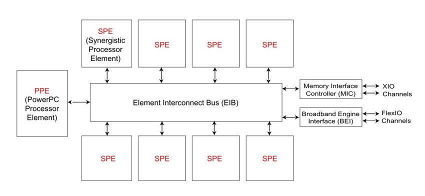
Experiments with a parallel WLMC code on the Isis computer at UPPMAX yielded
the results in Figure 7. We look at wall time required to reach an accurate solution
here because of course 10 processors will do 10 times the number of interactions,
but the problem mentioned above could be expected to harm the convergence rate.
The figure shows that this is not the case and performance is close to ideal.
Figure 7: Real runtime of parallel WLMC with varying number of processor cores compared to
ideal speedup
245 Conclusions
In this section, I will add some final thoughts and discuss the potential for fu-
ture work. While some technical challenges remain to be solved and only one
application was considered, the results are general enough to form the basis of
some broader conclusions regarding molecular simulations with electrostatics on
the PlayStation 3.
There is always a tradeoff to be made between usability and technical constraints.
The first attempt to create a library to accelerate the inverse-square root opera-
tion in existing Fortran programs was by far the most attractive from the users’
standpoint. With no need for additional programming, the most onerous com-
putational task would be speeded up by a factor of 6 compared to a SIMDized
sequential program. It sounds good, but Amdahl’s Law combined with the com-
putational overhead from parallelization and the slow PPU yielded a solution that
was much slower than even an unSIMDized x86 program. The goals of this im-
plementation were to check whether the computational overhead could be made
small enough to earn a small benefit and to learn how to code for the Cell, and
these goals were surely met despite the negative result.
The second attempt was more encouraging. The evaluation step for an MC code
is application-specific so a scientist would have to write SPE-enabled C code to
use a PS3, but related applications will have very similar evaluation steps. It is
conceivable that a family of PS3-specific MC evaluation routines could serve a
research group’s needs for quite some time, or that a scientist with a little C and
Cell experience could modify existing codes to address new simulations. However,
writing and debugging Cell code can challenge even a seasoned C programmer, so
until and unless the programming environment improves this solution is not ideal.
While the speed and scale of the third program was by far the best, this result is
diminished by a bug that remains unsolved. The mire of bit-shifting and sleights-
of-hand required to DMA, align, and iterate over a dozen buffers proved to be a
substantial obstacle that really held up progress. If a way could be found to alle-
viate this burden on the programmer, it would be well worth further investigation.
The final level of parallelization involving a cluster of PlayStation 3 machines was
in the end only subject to a theoretical investigation in this project. Other work
has shown that this is a promising idea and plays to the PS3’s strengths. The PS3
systems are a relatively cheap computational resource and the single-PS3 programs
show that it is possible to use that resource quite efficiently.
Given more time, it would be interesting first to write a working version of the
multi-PS3 code with a blocking scheme, and then to extend the program to treat
25scientifically interesting problems. This is not a trivial task, as two additional MC
moves would have to be introduced to deal with the counter-ions – translation and
clothed pivot. The current model also ignores bond energy, a problem which grows
only linearly with PE length and is therefore a relatively light computation but is
physically important.
The Sony PlayStation 3 is an exciting platform to work with, with a very different
character from other machines. It is well-suited for Monte Carlo simulations of
molecular systems involving electrostatics, although the path to a good implemen-
tation is difficult. The parallel Wang-Landau method has especially good chances
of utilizing the strengths of the PS3 as a tool for scientific computing without
suffering from its weaknesses.
26A Program Codes
Program 1 Basic polyelectrolyte MC program (pseudocode)
function main():
currentPoly = initialize()
while (! done)
pivot = randint(0,Nm-1)
newPoly = move(currentPoly, pivot)
if ( evaluate(currentPoly, newPoly, pivot) )
currentPoly = newPoly
end
function evaluate(current, new, pivot):
deltaE=0
for i=1:pivot (L1)
for j=pivot+1:end (L2)
temp[ind] = (current.x[i]-current.x[j])^2 +
(current.y[i]-current.y[j])^2 +
oldE = inv_sqrt(temp)
for i=1:pivot (L1)
for j=pivot+1:end (L2)
temp[ind] = (current.x[i]-new.x[j])^2 +
(current.y[i]-new.y[j])^2 +
(current.z[i]-new.z[j])^2
newE = inv_sqrt(temp)
for i=1:ind
deltaE += newE - oldE
if deltaProgram 2 PPE program for striping and blocking schemes (pseudocode)
function main():
currentPoly = initialize()
while ( ! done )
pivot = randint(0,Nm-1)
newPoly = move(currentPoly, pivot)
if ( evaluate(currentPoly, newPoly, pivot) )
currentPoly = newPoly
end
function evaluate(current, new, pivot):
// split work into parts, send to SPEs
start = 0
spes_left = num_spes
for ( i=0; iProgram 3 SPE program for blocking scheme (pseudocode)
function main():
while(! done)
delta = 0
work = wait_for_work()
! DMA first fixed block
! DMA first moved block of current poly
for i=0:numfixedblocks
! begin DMAing next fixed block
for j=0:nummovedblocks / 4
! begin DMAing next moved block of new poly
// calculate vector oldE
temp = (fixed.x[i]-moved.x[j])^2 +
(fixed.y[i]-moved.y[j])^2 +
(fixed.z[i]-moved.z[j])^2
oldE = inv_sqrt(temp)
! wait for DMA to complete
! begin DMAing next moved block of current poly
// calculate vector newE
temp = (fixed.x[i]-moved.x[j])^2 +
(fixed.y[i]-moved.y[j])^2 +
(fixed.z[i]-moved.z[j])^2
newE = inv_sqrt(temp)
for k=1:4
delta += newE[k] - oldE[k]
end
end
end
mail_to_PPU(delta)
end
29Program 4 PPE program for WLMC client (pseudocode)
function main():
currentPoly = initialize()
getInitialParametersFromServer()
while ( ! done )
for( i=0; iProgram 5 PPE program for WLMC server (pseudocode)
function main():
do
request = wait_for_client_connection()
if request == "updateUstar" then
newUstar = socket_read()
for i=1:numbins
myUstar[i] += newUstar[i]
end
if getPstarError < threshold then
dUstar = dUstar/2
socket_send(myUstar, dUstar)
else if request == "requestParameters" then
randomSeed = newSeed()
socket_send(initParams, myUstar, randomSeed)
while(! done)
31References
[1] Abraham Arevalo, Ricardo M. Matinata, Maharaja Pandian, Eitan Peri, Kur-
tis Ruby, Francois Thomas, and Chris Almond. Programming for the Cell
Broadband Engine. IBM Redbooks, 2008.
[2] Daan Frenkel and Berend Smit. Understanding Molecular Simulation: From
Algorithms to Applications. Academic Press, 2002.
[3] M. O. Khan and D. Y. C. Chan. Monte carlo simulations of stretched charged
polymers. In 4th International Symposium on Polyelectrolytes, pages 8131–
8139, Lund, Sweden, 2002. Amer Chemical Soc.
[4] M. O. Khan, G. Kennedy, and D. Y. C. Chan. A scalable parallel monte
carlo method for free energy simulations of molecular systems. Journal of
Computational Chemistry, 26(1):72–77, 2005.
[5] Malek O. Khan. Polymer Electrostatics: From DNA to Polyampholytes. PhD
thesis, Lund University, 2001.
[6] J. Kurzak, A. Buttari, P. Luszczek, and J. Dongarra. The playstation 3 for
high-performance scientific computing. Computing in Science and Engineering,
10(3):84–87, 2008. Kurzak, Jakub Buttari, Alfredo Luszczek, Piotr Dongarra,
Jack.
[7] N. Metropolis, A. W. Rosenbluth, M. N. Rosenbluth, A. H. Teller, and
E. Teller. Equation of state calculations by fast computing machines. J. Chem.
Phys., 21(6):1087–1092, June 1953.
[8] F. G. Wang and D. P. Landau. Efficient, multiple-range random walk algorithm
to calculate the density of states. Physical Review Letters, 86(10):2050–2053,
2001.
32You can also read