Job Growth from Opportunity Zones* - Alina Arefeva - American Economic ...
←
→
Page content transcription
If your browser does not render page correctly, please read the page content below
Job Growth from Opportunity Zones*

                             Alina Arefeva                                   Morris A. Davis
                   University of Wisconsin-Madison                            Rutgers University
                     Wisconsin School of Business                         Rutgers Business School

                      Andra C. Ghent                                                Minseon Park
       University of North Carolina - Chapel Hill                         University of Wisconsin-Madison
               Kenan-Flagler Business School

                                              November 16, 2020

                                                         Abstract
           The Tax Cuts and Jobs Act of 2017 established a new program called Oppor-
        tunity Zones (OZs) that created tax advantages for investing in businesses or
        real estate in a limited number of low-income Census tracts. We use a census of
        establishment-level data on employment to identify the effect of the program on
        job creation. We show that in metropolitan areas, the OZ designation increased
        employment growth relative to comparable tracts by between 3.0 and 4.5 per-
        centage points and new jobs were created across many different industries and
        education levels. The OZ designation did not create jobs in rural areas.

            Keywords: Placed-Based Policies, Opportunity Zones, Tax Incentives.
            JEL codes: H73, R30, R38, G11, G18.

     * Arefeva: arefeva@wisc.edu; Davis: mdavis@business.rutgers.edu; Ghent: andra ghent@kenan-flagler.unc.edu.; Park:
mpark88@wisc.edu. We thank Philip McDaniel, the UNC GIS librarian, for his assistance, Dan Hartley for sharing his data on
Census tract centroids and adjacent tracts, and Steve Malpezzi for helpful conversations. The paper has benefited from the feed-
back of workshop participants at the AREUEA 2020 Virtual Seminar Series, Peking University Guanghua School of Business
& Jinan University IESR, Rutgers University, the University of California - Santa Cruz, the University of North Carolina at
Chapel Hill, the University of Wisconsin-Madison, and the Urban Economics Association 2020 Annual Meeting. We are grateful
for the financial support of an award from the University of Wisconsin’s Fall Research Competition. We have been authorized to
use YTS through the Business Dynamics Research Consortium (BDRC) by the University of Wisconsin’s Institute for Business
and Entrepreneurship. The contents of this paper are solely the responsibility of the authors.
1        Introduction

The economic well-being of Americans varies dramatically across places, even within
the same Metropolitan Statistical Area (MSA). Localized pockets of poverty persist
and the convergence in economic fortunes that historically characterized the US econ-
omy has ceased in the last few decades (see, for example, Ganong and Shoag (2017)).
Mobility costs remain high, especially for low-income households that tend to live in
low-income communities, and mobility has decreased in recent years.1
        Against this backdrop, there is renewed interest in policies to promote employ-
ment in low-income places. Even researchers recently skeptical of place-based policies
now appear more open to potential benefits of these policies; compare, for example,
Austin, Glaeser, and Summers (2018) with Glaeser (2012). The Tax Cuts and Jobs
Act of 2017 introduced a new national place-based policy in the form of capital gains
tax relief to investments operating in particular low-income communities called Op-
portunity Zones (OZs). We study the impact of the OZ program on employment in the
small geographic areas, Census tracts, directly receiving the tax benefits as well as
surrounding areas.
        While the OZ program has the potential to create jobs in distressed communities,
there are a number of reasons to believe the program may not have any effects, or
perhaps even detrimental effects on employment. For example, depending on the
complementarity of capital and various types of labor, a decrease in capital gains
taxes has the potential to reduce labor demand. Additionally, given the US Federal
    1
    Topel (1986), Henderson and Ioannides (1989), Bound and Holzer (2000), and Hedman (2013),
among others, provide evidence that low-income households face higher mobility costs. Molloy, Smith,
and Wozniak (2011) review potential reasons for the recent decline in household mobility in the United
States.

                                                  1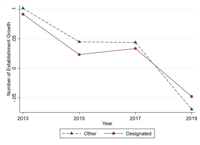
tax code already allows real estate investors to defer capital gains taxes via the 1031
exchange program, the OZ program may only reduce the taxes paid by inframarginal
investors rather than increasing the flow of capital to low-income communities. A
quantitative analysis is needed to estimate how many jobs the OZ program created
and to compare the program’s cost-effectiveness with other job-creation programs.
   We study the effect of the OZ program on job growth at the Census tract-level using
a difference-in-difference strategy that compares growth in tracts designated as OZs
with growth in tracts that were eligible but not designated as OZs. We show the OZ
program increased employment and establishment growth in tracts in metropolitan
areas receiving tax benefits by between 3 to 4.5 percentage points over the 2017-2019
period relative to similar, eligible tracts that were not chosen to receive benefits. In
contrast, we find tracts designated as OZs in non-metropolitan (rural) areas expe-
rienced no such job growth. While we find that state governors’ choice of tracts was
somewhat political, our results are unchanged when we control for the extent to which
a tract was chosen as part of a political process. Our results are robust to a placebo
test in which we use a counterfactual date for the designation.
   We show at least some of the jobs that were created were likely filled by lower-
skilled workers based on the average skill-level used in the industry. The construction
industry experienced the greatest job growth but jobs were also generated in trade
and service industries. Finally, we find that the program had significant positive
spillovers to employment and establishment growth in nearby tracts.
   A number of recent papers have studied the impact of the OZ program on vari-
ous outcomes of interest not related to employment, the focus of our paper. Chen,
Glaeser, and Wessel (2019) argue that the program did not significantly affect the

                                           2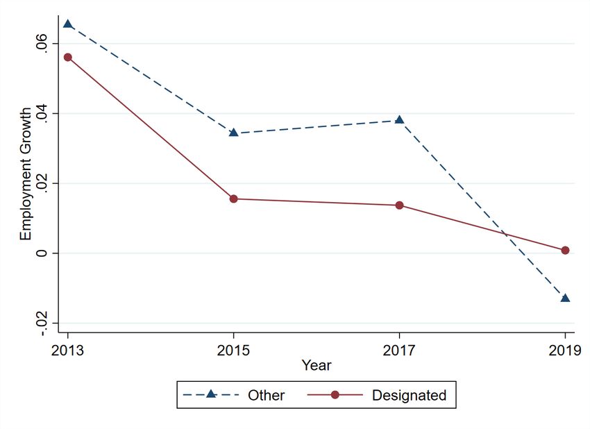
growth of single-family house prices. Sage, Langen, and Van de Minne (2019) show
prices increased for redevelopment properties and vacant sites, but the price of exist-
ing commercial properties did not rise. Perhaps the closest paper to ours is Atkins,
Hernández-Lagos, Jara-Figueroa, and Seamans (2020) who study job postings. These
authors find that the number of job postings linked to ZIP codes that include at least
one tract designated to receive tax benefits from the OZ program were lower than the
number of postings associated with ZIP codes that include no such tracts. Our mea-
surement of outcomes is employment, not postings, and our level of geography is the
Census tract, which exactly aligns with the geography in the OZ program legislation.
   We contribute to the literature on place-based policies, reviewed in Neumark and
Simpson (2015), by evaluating the impact of one of the biggest federal place-based
policies on local employment and establishment growth. To our knowledge, ours is
the first paper looking at the effects of a nationwide place-based policy on job growth
at the tract-level. Earlier national place-based programs in the US, Enterprise Com-
munities (ECs) and Renewal Communities (RCs), targeted a smaller number of tracts
and focused on providing wage credits, higher depreciation expense allowances, and
tax-exempt funding. Some prior research has failed to find significant effects of place-
based policies, for example, Neumark and Kolko (2010) who analyze California’s EC
program. More recent studies, such as Billings (2009) and Busso, Gregory, and Kline
(2013) of Empowerment Zones (EZ), Ham, Swenson, İmrohoroğlu, and Song (2011) of
EZs and state and federal ECs, and Freedman (2012) and Harger and Ross (2016) of
New Market Tax Credits (NMTCs), find a significant positive impact on local employ-
ment.
   Our paper is also related to a literature studying the effect of capital gains taxes

                                           3
on investor behavior. The majority of this literature uses data from publicly-traded
equities. Research topics include the effect of capital gains taxes on investor holding
periods (Ivković, Poterba, and Weisbenner, 2005; Dammon and Spatt, 2015; Dammon,
Spatt, and Zhang, 2015), stock prices (Dai, Maydew, Shackelford, and Zhang, 2008;
Lang and Shackelford, 2000; Starks, Yong, and Zheng, 2006), and corporate gover-
nance (Dimmock, Gerken, Ivković, and Weisbenner, 2018). Outside of publicly-traded
equities, Shan (2011), Heuson and Painter (2014), and Agarwal, Li, Qin, Wu, and
Yan (2020) find that capital gains taxes meaningfully affect individuals’ housing deci-
sions while Edwards and Todtenhaupt (forthcoming) show that the reduction of capi-
tal gains taxes in the US in 2010 increased funding for start-up firms. Poterba (2002)
hypothesizes that the effect of capital gains taxes will be smaller for investments like
commercial real estate than for publicly traded equities. We instead show that the
capital gains tax relief of the OZ program meaningfully increased construction em-
ployment in the targeted areas, suggesting that capital gains taxes can influence the
investment choices of investors in commercial real estate.
2 Identifying the Effect of the OZ Program
2.1 Background
The concept of tax-advantaged Opportunity Zones had bipartisan support and back-
ing, as the legislation was conceived and sponsored by Democratic Senator Corey
Booker and Republican Senator Tim Scott (Booker, 2019). The 2017 Tax Cut and
Jobs Act (TCJA), signed into law by President Trump on December 22, 2017, included
the OZ legislation with provisions of the law to apply to the 2018 tax year. The TCJA
4allowed state executives to designate up to 25% of low-income tracts and some tracts
contiguous with low-income tracts as OZs.2 The governors of each state designated
tracts from among those eligible in early 2018 and all states completed their designa-
tions by June 2018 (U.S. Department of the Treasury, 2018).
For the purposes of the OZ legislation, the definition of a low-income community
(LIC) is from section 45D(e) of the U.S. tax code (Internal Revenue Service, 2010) and
requires that the tract meet at least one of the following criteria:
1. A poverty rate of at least 20%,
2. The tract is not in a metropolitan area and median family income does not ex-
ceed 80% of statewide median family income,
3. The tract is in a metropolitan area and median family income is less than or
equal to 80% of the greater of metropolitan area or statewide family income,
4. The tract has a population of less than 2,000 people, it is within an empower-
ment zone, and it is contiguous to one or more LIC.
At least 95% of tracts designated to receive favorable OZ tax treatment had to be
an LIC as defined above. Additionally, the median income of any designated tract
contiguous to an LIC must be less than 125% that of the median income of the LIC
with which the tract is contiguous (US House of Representatives, 2017).
The OZ program includes two different types of tax relief for capital gains. First,
investors with realized capital gains on existing assets can defer paying tax on the
gains by investing them into existing or new businesses or newly constructed real
2
If the number of low-income tracts in a state is less than 100, a total of 25 tracts may be designated
(US House of Representatives, 2017).
5estate in designated OZ tracts. Abstracting from some details, taxes on the realized
capital gains from the prior investments can be deferred for seven years at which
point the taxable basis of the capital gains is reduced by 15% and the tax becomes
payable. Investors can either invest directly in an OZ or in a Qualified Opportunity
Fund (QOF). A QOF must invest at least 90% of its assets into existing or new busi-
nesses or newly constructed real estate in an OZs. Because of this transfer of capital
gains on old assets into a QOF, investors sometimes refer to the OZ program as the
“1031 exchange program on steroids”. Second, and perhaps most importantly, capital
gains on any new investments in an OZ are totally tax-free as long as the new in-
vestment is held for at least ten years. For additional details, see Internal Revenue
Service (2020) and US House of Representatives (2017).
Policy makers’ stated motivation for creating OZs was to spur job growth in ar-
eas left behind by the economic expansion. In particular, Republicans in the Senate
asserted the rationale for OZs as follows:
Although the post-recession U.S. economy has entered its 10th year of ex-
pansion, job and wage growth has been geographically uneven. Approxi-
mately 50 million Americans live in communities where the decline of in-
dustries like mining, manufacturing, and textiles has led to stubbornly
high rates of unemployment and poverty.
One significant handicap for these communities has been the lack of access
to loans, grants, and venture capital needed to start or expand a small
business. Opportunity zones were devised to address this gap. US Senate
Republican Policy Committee (2019)
Similarly, the Internal Revenue Service (2020) asserts that “[O]pportunity zones are
6an economic development tool - that is, they are designed to spur economic develop-
ment and job creation in distressed communities.” Treasury Secretary Steven Mnuchin
called the creation of OZs “one of the most significant provisions of the Tax Cut and
Jobs Act” and a provision that would stimulate job creation (U.S. Department of the
Treasury, 2018).
While policy makers did not clarify why they believed the market distribution
of economic activity across space was inefficient or inequitable, economists propose
several arguments for place-based policies; see Neumark and Simpson (2015) for an
overview. Perhaps the most compelling efficiency-based reason is that multiple equi-
libria may arise in models with agglomeration economies and a particular location
may be stuck in a bad equilibrium; see Kline (2010) for an illustration. Under this
rationale, a successful place-based policy would at a minimum increase employment.
Equity-based rationales for place-based policies similarly would suggest a minimum
requirement for a policy to be successful is for it to generate an increase in labor de-
mand, and the most frequently mentioned rationale for the policy by policy makers is
job creation (Internal Revenue Service, 2020; U.S. Department of the Treasury, 2018).
We thus assess the extent to which the OZ legislation achieved its stated goals.
2.2 Methodology
Similar to the approach Chen, Glaeser, and Wessel (2019) use to identify the effect
of the OZ program on house prices, we use a difference-in-difference (DiD) strategy
to identify the effect of the program on tract-level employment and establishment
growth. This method exploits the discretion left to state Governors to designate par-
ticular tracts for preferential tax treatment of the OZ program. While governors may
7have chosen tracts at least partially based on political considerations, such that desig-
nated tracts may differ systematically from those left undesignated, we include many
controls for fixed characteristics of tracts and perform a variety of analyses to show
that selected tracts and eligible-but-not-chosen tracts did not differ in unobserved
ways.
We compare two-year employment growth in tracts that were designated, tracts
we refer to as “Designated,” with tracts that were eligible to receive benefits based
on the criteria described in Section 2.1 but not chosen. We refer to the eligible-but-
not-chosen as “Other” tracts throughout. While all eligible tracts including those ulti-
mately designated satisfy the eligibility criteria, we capture systematic differences in
outcomes between Designated and Other tracts that are not absorbed by our control
variables by using a fixed effect for Designated. We also consider a specification in
which we include tract fixed effects and find extremely similar results to our bench-
mark specification.
All of our DiD analyses use the following regression specification
Yi,t = α0 + α1 Pt + α2 Di + α3 Di Pt + Xi αX + i,t (1)
where Yi,t is two-year growth in an economic variable of interest in the tract, Pt is
a dummy variable equal to 1 for the post-2017 period, 0 otherwise, Di is a dummy
variable that takes a value of 1 if the tract was Designated and 0 otherwise, and Xi is
a vector of characteristics of the tract that do not vary over the observation periods.
In our initial regressions, we include observations from 2015-2017 and 2017-2019 and
all tracts eligible to receive preferential tax treatment from the OZ legislation.3 We
3
The list of all eligible tracts and those ultimately designated is available at
8vary the sample dates, the set of tracts in the sample, and Yi,t and Xi to investigate
details and perform a variety of robustness tests.
2.3 Data
Our main dataset is establishment-level employment data from Your-economy Time
Series (YTS) and covers 2015-2019. Infogroup is the provider of the licensed database
used to create the Your-economy Time Series (YTS). We sum over establishments in
each eligible tract to generate two variables of interest at the tract-level: employment
and number of establishments. We then calculate two-year growth of each of these
outcomes when estimating equation (1).
The YTS data begins in 1997 and covers all US public and private establishments.
YTS aggregates data from the Infogroup Business Data historical files. Kunkle (2018)
details Infogroup’s methodology to gather the data underlying YTS:
To develop its datasets, Infogroup operates a 225-seat call center that makes
contact with over 55,000 businesses each and every day in order to record
and qualify company information. During a typical month, 15% of the en-
tire Infogroup business dataset is re-verified. On average, 150,000 new
businesses are added while 100,000 businesses are removed each month,
capturing the dynamic business churn happening in the economy. In-
fogroup’s team also identifies new companies through U.S. Yellow Pages,
county-level public sources on new business registrations, industry direc-
tories, and press releases.
https://edit.urban.org/sites/default/files/urbaninstitute_tractleveloz
analysis_update1242018.xlsx.
9Kunkle (2018) compares the YTS data with employment data from the US Bureau of
Labor Statistics (BLS). He finds that the YTS data is as encompassing as the data
in the Current Population Survey (CPS). Additional information on the YTS data are
available at https://wisconsinbdrc.org/data/.
For the regression covariates Xi , we use tract-level data from the 2013-2017 5-
year American Community Survey (ACS).4 We include the share of the population
that is white, the share with higher education, the share that rent, the share living
in poverty, the share covered by health insurance among native-born individuals, the
log of median annual earnings, the log of median annual household income, the log of
median monthly gross rent, the share of households receiving supplemental income,5
the average daily commute time, and the share of the population that is employed.
Table 1 summarizes the data in our preliminary, unrestricted sample of all eligible
tracts. We highlight here a few points from the table. First, the average population
was 4,172 people and the average poverty rate was 19%. Second, establishments
located in tracts in this sample employed 2,148 workers, on average, although only
29.7% of the resident population of these tracts was employed. Finally, the rightmost
column of Table 1 highlights the presence of outlier tracts with extreme values for
employment and establishment growth. We adopt various strategies that we discuss
later to address the impact of outliers on results.
Table 2 reports these same variables separately for Designated and Other tracts.
Consistent with the presumption that state executives used the OZ program to benefit
4
Source: https://www.census.gov/data/developers/data-sets/acs-5year/2017.html. Table 12 in the
Appendix lists the full set of ACS control variables we include in our regressions; we use the same
set of ACS control variables as Chen, Glaeser, and Wessel (2019).
5
Supplemental income includes food stamps/Supplemental Nutrition Assistance Program (SNAP),
public assistance income, or Supplemental Security Income (SSIP).
10the maximum number of people, employment and the number of establishments are
substantially higher in Designated than in Other tracts. Other tracts had an average
of 1,912 employees while Designated tracts had average employment of 3,156 peo-
ple. Designated tracts also have a higher poverty rate (25% vs. 18%), lower median
household income, lower median earnings, less education, and a higher percentage of
non-white residents than Other tracts. While Designated tracts are larger in terms
of employment and the number of establishments than the Other tracts, they expe-
rienced lower growth in employment and the number of establishments in the two
years prior to the passage of the TCJA.
As a precursor to our formal DiD analysis, Figure 1 shows average growth rates
for employment and the number of establishments in Designated and Other tracts.
The top two graphs display the raw data; the bottom two graphs show the data after
winsorizing at the 1% level to address the influence of outliers. All graphs show four
growth rates: 2011-2013, 2013-2015, 2015-2017 and 2017-2019 labeled, respectively,
as 2013, 2015, 2017 and 2019. All graphs show that growth rates of Designated and
Other tracts had similar but not identical trends prior to the TCJA, with Other tracts
having higher rates of growth for both employment and establishments up through
2017. The positive effect of the TCJA on growth in Designated tracts from 2017-
2019 is quite visible in the bottom two figures, a finding we confirm in our regression
analyses.
11Table 1: 2017 Characteristics of Eligible Tracts
Variable Obs. Mean SD Median Minimum Maximum
Designated 41,174 0.190 0.392 0 0 1
Number of entered establishments 41,174 48.7 70.6 30 0 2,456
Number of exited establishments 41,161 43.4 67.9 28 0 4,709
Percent of entered establishments 41,161 0.279 0.215 0.224 0 9
Percent of exited establishments 41,161 0.235 0.094 0.216 0 1
Number of establishments 41,174 202 266 130 1 12793
Growth in the number of establishments 41,161 0.044 0.180 0.016 -0.864 9
Employment 41,174 2,148 4,013 1,137 1 235,158
Employment growth 41,161 0.039 0.349 0.014 -0.985 41.1
Total housing 41,164 1,534 707 1,446 0 12,768
% White 41,146 0.659 0.280 0.735 0 1
% Higher ed 41,146 0.191 0.104 0.173 0 1
% Renters 41,107 0.455 0.227 0.426 0 1
% Native-born with health insurance 41,139 0.891 0.060 0.901 0 1
% Poverty 41,146 0.190 0.103 0.170 0 1
% Supplemental income 41,146 0.092 0.064 0.079 0 0.528
% Employed 41,146 0.297 0.078 0.3 0 1
Median annual earnings 41,058 $27,384 $7,929 $26,772 $2,499 $116,354
Median annual household income 41,029 $44,553 $15,531 $43,077 $2,499 $177,824
Median monthly gross rent 40,917 $899 $308 $832 $99 $3,501
Population 41,164 4,172 1,994 3,905 0 40,402
Average daily commuting time (min) 26,190 36.9 14.8 34.9 3.3 632.5
Notes: 1) Growth in employment and the number of establishments is measured
over the two-year 2015-2017 period.
12Table 2: 2017 Characteristics of Eligible Tracts by Designation
Variable Mean SE t-value for
Other Designated Other Designated diff. in means
Designated 0 1 0 0
Number of entered establishments 46.2 59.4 66.8 84.0 -15.0
Number of exited establishments 40.7 55.2 63.9 81.7 -17.1
Percent of entered establishments 0.284 0.259 0.210 0.234 9.11
Percent of exited establishments 0.238 0.221 0.095 0.085 14.4
Number of establishments 186 269 244 334 -25.1
Growth in the number of establishments 0.046 0.038 0.171 0.213 3.41
Employment 1912 3156 3589 5349 -24.8
Employment growth 0.044 0.019 0.362 0.285 5.825
Total housing units 1550 1464 711 687 9.73
% White 0.680 0.574 0.271 0.299 30.4
% Higher ed 0.198 0.160 0.106 0.090 29.3
% Renters 0.432 0.552 0.222 0.224 -42.9
% Native-born with health insurance 0.894 0.879 0.058 0.064 20.0
% Poverty 0.177 0.246 0.097 0.110 -55.3
% Supplemental income 0.086 0.119 0.060 0.072 -41.8
% Employed 0.303 0.268 0.077 0.077 36.8
Median annual earnings $28,087 $24,386 $7899 $7335 37.7
Median annual household income $46,435 $36,538 $15,444 $13,167 52.3
Median monthly gross rent $915 $826 $314 $271 23.1
Population 4208 4022 1997 1973 7.5
Average daily commuting time (min) 36.8 14.7 37.1 15.2 -1.11
Notes: 1) Growth in employment and the number of establishments is measured
over the two-year 2015-2017 period.
13Figure 1: Biennial Tract Growth Rates for Eligible Tracts
(a) Employment Growth, Raw Data (b) Establishment Growth, Raw Data
(c) Employment Growth, Winsorized at 1% (d) Establishment Growth, Winsorized at 1%
143 Results
3.1 All eligible tracts
Table 3 presents DiD results for employment (panel A) and establishment growth
(panel B). In columns (1) and (3), we include all observations in the sample. In column
(1) we include no controls while column (3) includes lagged growth (i.e. growth from
2013-2015) of the dependent variable as well as the full set of tract-level controls
from the ACS. For employment growth in panel A, the coefficient on the interaction
between Di and Pt is 0.025 in column 1 and 0.028 in column 3, indicating the OZ
program boosted employment growth by about 2.5 percentage points in Designated
tracts, although the point estimates are not statistically significant as the standard
errors are large. Panel B shows the estimates of the OZ program on establishment
growth. The program increased establishment growth by 2.1 - 2.2 percentage points,
shown in columns 1 and 3; these estimates are statistically significant.
15Table 3: Employment and Establishment Growth Regressions
(1) (2) (3) (4) (5) (6) (7) (8) (9) (10)
OLS LAV OLS LAV OLS OLS OLS GLS FE OLS
Winsorized at Winsorized at 1%
0.5% 1% 2.5% Weighted CBSA FE SEs Clustered
ACS Controls No No Yes Yes Yes Yes Yes Yes Yes Yes
No. of CBSAs 928
Panel A: Employment Growth
Designatedi -0.027* -0.015*** -0.018 -0.009*** -0.012** -0.012*** -0.012*** -0.006* -0.012*** -0.012***
(0.015) (0.003) (0.015) (0.003) (0.005) (0.005) (0.004) (0.003) (0.005) (0.004)
P ostt 0.001 -0.072*** -0.003 -0.074*** -0.043*** -0.050*** -0.059*** -0.079*** -0.053*** -0.050***
(0.009) (0.002) (0.009) (0.002) (0.003) (0.003) (0.002) (0.002) (0.003) (0.012)
Designatedi P ostt 0.025 0.021*** 0.028 0.021*** 0.038*** 0.036*** 0.033*** 0.018*** 0.036*** 0.036***
(0.022) (0.004) (0.021) (0.004) (0.007) (0.006) (0.005) (0.005) (0.006) (0.008)
Emp.Growth2013−2015 0.098*** -0.003 0.016*** 0.009* 0.003 -0.058*** 0.005 0.009
(0.017) (0.004) (0.006) (0.005) (0.004) (0.003) (0.005) (0.010)
Observations 52,060 52,060 52,053 52,053 52,053 52,053 52,053 52,053 52,053 52,053
16
R2 0.000 0.002 0.008 0.010 0.018 0.035 0.010 0.010
Panel B: Establishment Growth
Designatedi -0.007 -0.005* -0.007 -0.006** -0.009*** -0.008*** -0.008*** -0.010*** -0.008*** -0.008*
(0.007) (0.003) (0.007) (0.003) (0.003) (0.003) (0.003) (0.002) (0.003) (0.005)
P ostt -0.097*** -0.091*** -0.098*** -0.093*** -0.110*** -0.109*** -0.103*** -0.104*** -0.112*** -0.109***
(0.004) (0.002) (0.004) (0.002) (0.002) (0.002) (0.002) (0.002) (0.002) (0.016)
Designatedi P ostt 0.021** 0.020*** 0.022** 0.018*** 0.030*** 0.030*** 0.026*** 0.019*** 0.029*** 0.030***
(0.010) (0.004) (0.010) (0.004) (0.004) (0.004) (0.004) (0.003) (0.004) (0.009)
Emp.Growth2013−2015 0.127*** 0.016*** 0.024*** 0.021*** 0.018*** 0.012*** 0.015*** 0.021***
(0.008) (0.003) (0.004) (0.003) (0.003) (0.002) (0.003) (0.006)
Observations 52,060 52,060 52,053 52,053 52,053 52,053 52,053 52,053 52,053 52,053
R2 0.011 0.018 0.071 0.080 0.091 0.117 0.081 0.080
Notes: 1) Columns (2) and (4) report results for quantile regression to the median or Least Absolute Value (LAV). 2) Weight
for column (8) is 2015 Census tract employment. 3) In column (10), standard errors are clustered by CBSA. 4) Standard
errors in parentheses. 5) ***, **, and * denote significance at the 1%, 5%, and 10% levels. 6) Emp.Growth2013−2015 is the
growth in tract employment from 2013 to 2015. 7) Pt is a dummy variable equal to 1 for the post-2017 period, 0 otherwise, Di
is a dummy variable that takes a value of 1 if the tract was designated an OZ and 0 otherwise.As the summary statistics in Table 1 illustrate, our data contains extreme outliers
in some tracts and these may disproportionately affect standard errors. In columns
(2) (no controls) and (4) (full set of ACS controls) we run Least Absolute Variation
regressions i.e., regressions to the median, to mitigate the influence of outliers. Ac-
cording to these specifications, the effect of the OZ program on employment and es-
tablishments is positive and highly statistically significant. The point estimates in
both columns (2) and (4) indicate that the program raised employment growth by 2.1
percentage points and increased the growth in the number of establishments by 1.8 -
2.0 percentage points.
Columns (5) through (7) present the OLS results when we winsorize the dependent
variable at the 0.5%, 1%, and 2.5% levels and include all ACS controls. The results are
broadly similar regardless of the level at which we winsorize: these estimates suggest
the program increased employment by approximately 3.6 percentage points and the
number of establishments by approximately 3 percentage points. For both dependent
variables and for all three levels of winsorization, the coefficient on the interaction
between Di and Pi is statistically significant at the 1% level. In the remainder of our
analyses, we winsorize the dependent variable at the 1% level whenever we run OLS
regressions.
In column (8), we weight the observations by the total employment in the tract in
2015. Weighting by employment reduces the magnitude of the effect on employment
to 1.8 percentage points from 3.6 percentage points in our benchmark specification
(column (6)), suggesting that the program disproportionately affected less populous
tracts.6 In column (9), we include core-based statistical area (CBSA) fixed effects
6
Indeed, in binned regression analyses (not reported), we find larger effects for less populous tracts.
Similarly, when we weight by tract population instead of employment, also not reported, the effect of
17while column (10) clusters the standard errors by CBSA. The estimates are similar
(with slightly larger standard errors in the case of clustering by CBSA) to the specifi-
cation when we simply winsorize at 1%, column (6).
Our preferred regression specifications correspond to columns (4) and (6), LAV and
OLS with winsorizing at 1%. For the rest of the analysis, we will focus on these two
specifications.
3.2 Metropolitan versus non-metropolitan areas
Columns (1) and (2) of Table 4 show our benchmark specifications for the sample of el-
igible tracts located in metropolitan areas. The estimated effects on employment and
establishment growth are 2.9 - 4.6 percentage points, higher than the estimates for all
eligible tracts reported earlier. Columns (3) and (4) report the results for the sample
of eligible tracts outside of metropolitan areas. For tracts in non-metropolitan areas,
the results are different: The estimate of the OZ program on employment growth is
essentially zero and the estimate on establishment growth is negative. This latter
result is our only significant and economically meaningful negative finding of the OZ
program on growth. Since we are mostly concerned about employment growth, we
conclude that the OZ program had little to no impact on growth in tracts that are
not located in metropolitan areas and we drop these tracts from our sample in all
analyses that follow. We refer to the metropolitan-area sample of tracts and specifi-
cations in columns (1) and (2) as our “benchmark specifications” for the remainder of
the paper.
the program on the number of establishments declines.
18Table 4: Employment and Establishment Growth Within and Outside of Metro Areas
(1) (2) (3) (4)
LAV OLS LAV OLS
Winsorized at 1% Winsorized at 1%
ACS Controls Yes Yes Yes Yes
Metropolitan Area Non-Metropolitan Area
Panel A: Employment Growth
Di -0.014*** -0.019*** 0.008 0.015
(0.003) (0.005) (0.007) (0.012)
Pt -0.091*** -0.077*** -0.016*** 0.044***
(0.002) (0.003) (0.004) (0.007)
Di Pt 0.029*** 0.046*** -0.012 -0.000
(0.005) (0.007) (0.010) (0.015)
Emp.Growth2013−2015 -0.005 -0.005 0.021*** 0.048***
(0.004) (0.006) (0.007) (0.011)
Observations 40,944 40,944 11,109 11,109
R2 0.020 0.017
Panel B: Establishment Growth
Di -0.014*** -0.016*** 0.016*** 0.024***
(0.003) (0.003) (0.006) (0.007)
Pt -0.117*** -0.140*** -0.015*** 0.003
(0.002) (0.002) (0.003) (0.004)
Di Pt 0.032*** 0.043*** -0.022*** -0.023**
(0.004) (0.005) (0.007) (0.009)
Emp.Growth2013−2015 0.010*** 0.015*** 0.045*** 0.039***
(0.004) (0.004) (0.005) (0.007)
Observations 40,944 40,944 11,109 11,109
R2 0.125 0.011
Notes: 1) Columns (1) and (3) report results for quantile regression to the median or
Least Absolute Value (LAV). 2) Standard errors in parentheses. ***, **, and * denote
significance at the 1%, 5%, and 10% levels. 4) Emp.Growth2013−2015 is the growth in
tract employment from 2013 to 2015. 5) Pt is a dummy variable equal to 1 for the
post-2017 period, 0 otherwise, Di is a dummy variable that takes a value of 1 if the
tract was designated an OZ and 0 otherwise.
193.3 Robustness
3.3.1 LICs
A tract is eligible to be designated if it is an LIC or if it is contiguous to an LIC
(non-LIC). We identify whether the effect of the program differs for LIC and non-
LIC tracts by running the DiD regression (1) separately for the LIC and non-LIC
tracts. Columns (1) and (2) of Table 5 show the results for tracts eligible by the LIC
criteria. LIC tracts experienced similar growth in employment and establishments
as the overall sample of all tracts in metropolitan areas, between 3.3 - 5.0 percentage
points. Columns (3) and (4) repeat this analysis for tracts eligible by the contiguity
criteria (non-LIC). Our point estimates suggest these tracts experienced much faster
employment growth, 12.4 - 13.3 percentage points, and much faster establishment
growth, 8.2 - 8.8 percentage points. However, the standard errors on these estimates
are also higher.7
7
Recall that no more than 5% of the Designated tracts could be designated by the contiguity cri-
teria, which reduced the non-LIC sample size to around 4,910 tracts out of which around 89 were
designated. The number of observations in column (3) of table 5, 9,510, is equal to two times 4,910 less
310 observations from 155 tracts where we do not have information on commuting time.
20Table 5: Robustness
(1) (2) (3) (4) (5) (6) (7) (8) (9) (10)
LIC Non-LIC 3-mile Ring LIC + 3-mile Ring Placebo
LAV OLS LAV OLS LAV OLS LAV OLS LAV OLS
Winsorized at 1% Winsorized at 1% Winsorized at 1% Winsorized at 1% Winsorized at 1%
Panel A: Employment Growth
Di -0.015*** -0.023*** -0.005 0.004 -0.015*** -0.023*** -0.016*** -0.020*** -0.008*** -0.012***
(0.004) (0.005) (0.022) (0.029) (0.004) (0.005) (0.004) (0.004) (0.002) (0.003)
Pt -0.094*** -0.084*** -0.077*** -0.058*** -0.102*** -0.098*** -0.129*** -0.155*** 0.007*** 0.007***
(0.002) (0.003) (0.004) (0.006) (0.003) (0.004) (0.003) (0.003) (0.001) (0.002)
D i Pt 0.033*** 0.050*** 0.133*** 0.124*** 0.040*** 0.064*** 0.041*** 0.055*** -0.006** -0.007
(0.005) (0.007) (0.032) (0.041) (0.005) (0.007) (0.005) (0.005) (0.003) (0.004)
Emp.Growth2013−2015 -0.006 -0.008 -0.003 0.001 -0.014*** -0.022*** 0.003 0.003 -0.013*** -0.024***
(0.005) (0.007) (0.010) (0.012) (0.005) (0.007) (0.005) (0.005) (0.002) (0.003)
Observations 31,434 31,434 9,510 9,510 27,543 27,543 27,543 27,543 41,926 41,926
R2 0.021 0.016 0.027 0.141 0.029
21
Panel B: Establishment Growth
Di -0.014*** -0.017*** -0.010 -0.016 -0.015*** -0.023*** -0.015*** -0.019*** -0.011*** -0.016***
(0.003) (0.003) (0.020) (0.019) (0.004) (0.005) (0.004) (0.004) (0.002) (0.003)
Pt -0.119*** -0.143*** -0.110*** -0.133*** -0.103*** -0.098*** -0.128*** -0.153*** 0.003* 0.004**
(0.002) (0.002) (0.004) (0.004) (0.003) (0.004) (0.003) (0.003) (0.001) (0.002)
D i Pt 0.033*** 0.045*** 0.082*** 0.088*** 0.040*** 0.062*** 0.040*** 0.053*** 0.006* 0.007*
(0.005) (0.005) (0.028) (0.027) (0.005) (0.008) (0.005) (0.005) (0.003) (0.004)
Emp.Growth2013−2015 0.009** 0.014*** 0.029*** 0.018** -0.008 -0.021*** 0.003 0.004 0.005** 0.015***
(0.004) (0.005) (0.008) (0.008) (0.005) (0.008) (0.005) (0.005) (0.002) (0.002)
Observations 31,434 31,434 9,510 9,510 23,580 23,580 23,580 23,580 41,926 41,926
R2 0.125 0.127 0.026 0.136 0.072
Notes: 1) Sample of tracts in metropolitan areas. 2) Columns (1), (3), (5), (7), (9) report results for quantile regression to the
median or Least Absolute Value (LAV). 3) Standard errors in parentheses. 4) ***, **, and * denote significance at the 1%, 5%,
and 10% levels. 5) Emp.Growth2013−2015 is the growth in tract employment from 2013 to 2015. 6) Di is a dummy variable that
takes a value of 1 if the tract was designated an OZ and 0 otherwise. 7) In columns (1)-(8), Pt is a dummy variable equal to 1
for the post-2017 period, 0 otherwise, In columns (9) and (10), Pt is equal to 1 for the 2015-2017 period, 0 otherwise.3.3.2 Nearby tracts
In this section we restrict the control group to non-selected eligible tracts located
within 3 miles of designated OZ tracts. We measure the distance between the cen-
troids of two tracts using the Haversine formula with radius 6,371. The treatment
group consists of Designated tracts, as before. By restricting tracts in the control
group to be geographically near non-selected eligible tracts, we hope to control for any
unobserved local economic forces. Columns (5) and (6) of Table 5 show estimates from
this restricted sample. The point estimates are a bit higher than the results shown
in Section 3.2, as they suggest employment and establishment growth increased by
4.0 - 6.4 and 4.0 - 6.2 percentage points, respectively. These estimates are robust to
further restricting the sample to LIC tracts, as can be seen in columns (7) and (8).
3.3.3 Placebo test
We check the robustness of our results by running a placebo test in which we pretend
that legislation for the OZ program occurred in 2015. In implementing the DiD, we
compare employment and establishment growth from 2015-2017 with 2013-2015 for
Designated tracts relative to Other tracts in metropolitan areas. Columns (9) and (10)
of Table 5 report the results. The point estimates of the coefficient on the interaction
term Di Pt are nearly zero and negative for employment growth and nearly zero and
positive but small for establishment growth, and only the small negative coefficient
on employment growth in the median regression (column 9) is statistically significant
at a 5% level. We conclude the results of this placebo test reinforce the validity of our
findings of a positive impact of the OZ designation on employment and establishment
growth in tracts in metropolitan areas.
223.3.4 Political tract selection
Perhaps not surprisingly, Frank, Hoopes, and Lester (2020) find that the process for
selecting specific tracts to receive preferential tax treatment arising from the OZ leg-
islation is somewhat political. To estimate whether this aspect of tract selection af-
fects our results, we collect data on the party of the state Governor and lower house
state legislators in 2018. We assign legislators to tracts using the lower chamber
State Legislative District Block Equivalent File. As in Frank, Hoopes, and Lester
(2020), we define a tract to be politically affiliated with the governor if the tract’s
lower house representative and the governor belong to the same party.
Many tracts belong to one electoral district, which sends one representative to the
lower house. In this case, a tract is represented by one lower house representative
and we set the variable defining whether the political affiliation of the tract is the
same as the governor, %sameparty, equal to 1 if the lower house representative and
the governor are in the same party, 0 otherwise. However, some tracts belong to sev-
eral electoral districts. Moreover, in some states, each electoral district sends two or
more representatives to the lower house. 10 U.S. states had multi-member districts
as of 2018. In these cases, a tract may have multiple lower house representatives. To
capture these cases, we set %sameparty equal to the share of the tract’s lower house
representatives that belong to the same party as the governor to measure political
affiliation of the tract. Out of 41,055 tracts included in the analysis, 12,094 (29%)
are matched with more than two legislators. As an alternative specification, we also
construct the variable N sameparty that simply counts the number of legislators rep-
resenting that tract of the same party as the governor.
Table 6 presents the estimates of a Linear Probability Model in which we check to
23see if tract political affiliation is predictive of a tract’s Designation as an OZ, condi-
tional on the tract being eligible. Columns 1 and 2 show results with the entire sample
(inclusive of non-metropolitan tracts) with state fixed effects but no ACS controls for
the two definitions of political affiliation. As in Frank, Hoopes, and Lester (2020),
tract political affiliation and designation as an OZ is negatively correlated without
controlling for tract observable characteristics. Columns 3 and 4 add ACS controls
to columns 1 and 2; these columns show that political affiliation and OZ designation
are significantly positively correlated once we control for observable tract attributes.
Finally, columns 5 and 6 are the same as 3 and 4, but with all non-metropolitan
tracts removed from the sample. With this sample restriction, the point estimates
fall slightly from those in columns 3 and 4, and the coefficient on N sameparty is no
longer statistically significant at the 5% level.
Column (1) and (2) of Table 7 show that the point estimates in Section 3.2 are
robust to controlling for the political affiliation of the tract, the sameparty variable.
In columns (3) and (4), we include an interaction of the sameparty variable with the
Pt and Di to see if the measured effect of the OZ program depends on the politi-
cal affiliation of the tract. The estimate on this triple interaction term is negative
and significant for employment growth; the estimate on the triple interaction term is
small and insignificant for the establishment growth.
3.4 Heterogeneity
Having demonstrated that the OZ program significantly and positively affected em-
ployment and establishment growth in designated tracts, we turn now to understand-
ing what type of employment and establishments the program created.
24Table 6: OZ selection and Political Consideration
(1) (2) (3) (4) (5) (6)
ACS Controls No No Yes Yes Yes Yes
State FE Yes Yes Yes Yes Yes Yes
Metropolitan Area
N sameparty -0.009*** 0.009** 0.007*
(0.003) (0.004) (0.004)
%sameparty -0.011*** 0.017*** 0.012**
(0.004) (0.005) (0.006)
Observations 41,055 41,055 25,920 25,920 20,890 20,890
R2 0.003 0.003 0.099 0.099 0.101 0.101
3.4.1 New or old establishments?
The regression results reported in Table 4 considered the net change in establish-
ments. Here, we consider establishment births and deaths. Table 8 shows that, rel-
ative to Other tracts, Designated tracts experienced a reduction in the number of
failing establishments, columns (3) and (4), and an increase in new establishments,
columns (1) and (2). The table shows that the effect of the OZ program on establish-
ment births is four to six times larger than the effect on establishment deaths.
3.4.2 Intensive or extensive margin?
We now study whether the OZ policy induced employment growth by encouraging
the growth of existing establishments (intensive margin) or new establishments (ex-
tensive margin). To address this question, we employ three definitions of “existing”
establishments. Group 1 includes establishments that existed in all years of the sam-
ple, i.e., 2013, 2015, 2017, and 2019. Group 2 includes establishments that existed
in 2015, 2017, and 2019. Finally, Group 3 includes all establishments that existed in
25Table 7: Employment and Establishment Growth with Political Consideration
(1) (2) (3) (4)
LAV OLS LAV OLS
Winsorized at 1% Winsorized at 1%
ACS Controls Yes Yes Yes Yes
Panel A: Employment Growth
Di -0.014*** -0.019*** -0.014*** -0.019***
(0.004) (0.005) (0.004) (0.005)
Pt -0.093*** -0.077*** -0.093*** -0.077***
(0.002) (0.003) (0.002) (0.003)
Di Pt 0.031*** 0.046*** 0.037*** 0.058***
(0.005) (0.007) (0.006) (0.009)
%sameparty 0.001 0.004 0.002 0.006*
(0.002) (0.003) (0.002) (0.003)
Di Pt %sameparty -0.011 -0.024**
(0.007) (0.010)
Emp.Growth2013−2015 -0.014*** -0.010* -0.013*** -0.010*
(0.004) (0.006) (0.004) (0.006)
Observations 40,716 40,716 40,716 40,716
R2 0.023 0.024
Panel B: Establishment Growth
Di -0.011*** -0.016*** -0.011*** -0.016***
(0.003) (0.003) (0.003) (0.003)
Pt -0.119*** -0.141*** -0.119*** -0.141***
(0.002) (0.002) (0.002) (0.002)
Di Pt 0.032*** 0.043*** 0.031*** 0.040***
(0.004) (0.005) (0.006) (0.006)
%sameparty 0.001 0.002 0.001 0.001
(0.002) (0.002) (0.002) (0.002)
Di Pt %sameparty 0.002 0.005
(0.006) (0.006)
Emp.Growth2013−2015 0.000 0.007* -0.000 0.007*
(0.004) (0.004) (0.004) (0.004)
Observations 40,716 40,716 40,716 40,716
R2 0.140 0.140
Notes: 1) Sample of tracts in metropolitan areas. 2) Columns (1), (3) report results for quantile
regression to the median or Least Absolute Value (LAV). 3) Standard errors in parentheses. 4) ***, **,
and * denote significance at the 1%, 5%, and 10% levels. 5) Emp.Growth2013−2015 is the growth in
tract employment from 2013 to 2015. 6) Pt is a dummy variable equal to 1 for the post-2017 period, 0
otherwise, Di is a dummy variable that takes a value of 1 if the tract was designated an OZ and 0
otherwise. 26Table 8: Establishment Birth and Death Regressions
(1) (2) (3) (4)
Percent of Entered Establishment Percent of Exiting Establishment
LAV OLS LAV OLS
Winsorized at 1% Winsorized at 1%
ACS Controls Yes Yes Yes Yes
Di -0.025*** -0.031*** -0.012*** -0.011***
(0.003) (0.003) (0.002) (0.002)
Pt -0.056*** -0.089*** -0.014*** -0.008***
(0.002) (0.002) (0.001) (0.001)
D i Pt 0.031*** 0.040*** -0.005* -0.009***
(0.004) (0.004) (0.003) (0.002)
Emp.Growth2013−2015 0.083*** 0.104*** 0.150*** 0.112***
(0.003) (0.003) (0.002) (0.002)
Observations 40,944 40,944 40,944 40,944
R2 0.177 0.211
Notes: 1) Sample of tracts in metropolitan areas. 2) Columns (2) and (4) report
results for quantile regression to the median or Least Absolute Value (LAV). 3)
Standard errors in parentheses. ***, **, and * denote significance at the 1%, 5%, and
10% levels. 4) Emp.Growth2013−2015 is the growth in tract employment from 2013 to
2015. 5) Pt is a dummy variable equal to 1 for the post-2017 period, 0 otherwise, Di
is a dummy variable that takes a value of 1 if the tract was designated an OZ and 0
otherwise.
27Figure 2: Estimates with Existing Establishments
Notes: 1) Sample of tracts in metropolitan areas. 2) ***, **, and * denote significance
at the 1%, 5%, and 10% levels. 3) See definitions of Intensive 1, 2, 3 in the text. 4)
The benchmark results are from column (2) of Table 4, OLS Winsorized at 1%.
2015, 2017, and 2019 and remained in the same tract in all three years.
Figure 2 presents the results for each of the definitions. Each shows the coefficient
estimate on Di Pt , the key interaction term; the blue bars show growth of employment
and the red bars show growth in establishments. Given that we restrict the sample
to establishments that existed before 2017, any establishment growth we estimate
in OZ tracts is driven by establishments that move across tracts. By definition, we
28cannot see the effect on establishment growth at the tract-level for the third group.
Summarizing the results of Figure 2, the blue bars show the effect of the OZ policy on
employment growth of existing establishments is positive but smaller than our base-
line estimates and insignificant while the red bars show that results for establishment
growth are essentially zero. Thus, the creation of new establishments is largely the
driving force of the positive effect of the OZ program on employment growth.
3.4.3 Which industries are affected?
We now turn to tract employment and establishment growth by industry type. We use
the classification of Mian and Sufi (2014) that is based on 4-digit NAICS industries.
We winsorize all dependent variables at 1% and run the DiD specifications separately
for establishments in the Construction, Non-tradable, Others, and Tradable sectors.
The Others category includes a variety of industries that Mian and Sufi (2014) do not
classify as tradable or non-tradable.
Figure 3 shows estimates of the impact of the OZ program on each sector. Like Fig-
ure 2, the blue bars show coefficient estimates on the interaction term for employment
growth and the red bars show coefficient estimates for establishment growth. This
figure shows that the OZ program had the largest impact on both employment and
establishment growth in the construction industry. Employment growth is lowest in
Non-tradable industries and establishment growth is lowest in Tradable industries.
Figure 3 suggests the OZ program may have largely created only construction
jobs. To investigate this possibility, we rerun our benchmark DiD specification but
exclude establishments in Construction industries. The estimates from this restricted
sample decline to 2.8 - 4.5 for employment growth and 3.3 - 4.3 percentage points for
29establishment growth, but remain statistically significant (not shown).
Figure 3: Estimates by Industry Type
Notes: 1) Sample of tracts in metropolitan areas. 2) Benchmark estimate is from
Table 4, column (2). 3) ***, **, and * denote significance at the 1%, 5%, and 10%
levels.
We also look at tract employment and establishment growth by 1-digit NAICS sec-
tors. Shown in Table 9, we aggregate 2-digit NAICS sectors into six broad sectors
that represent (1) agriculture, (2) construction, (3) manufacturing, (4) trade, (5) infor-
mation, FIRE (finance, insurance and real estate) and management, and (6) services.
Then we estimate the impact on employment and establishment growth for each 1-
digit NAICS sector. Figure 4 shows estimates with the dependent variable winsorized
30at the 1% level. The estimates for NAICS sectors 2 and 5, construction and informa-
tion, FIRE and management, are quite a bit higher than our benchmark estimates;
the response of the employment and establishment growth in NAICS sectors 4 and 6,
trade and services, are close to our benchmark results; and the response of employ-
ment and establishment growth is insignificant for agriculture and manufacturing,
NAICS sectors 1 and 3.
Table 9: One digit NAICS industries
2-digit 1-digit
NAICS Description NAICS
Sectors Sectors
Agriculture, Forestry, Fishing and Hunting (not covered in
11 1
economic census)
21 Mining, Quarrying, and Oil and Gas Extraction
22 Utilities 2
23 Construction
31-33 Manufacturing 3
42 Wholesale Trade
44-45 Retail Trade 4
48-49 Transportation and Warehousing
51 Information
52 Finance and Insurance
53 Real Estate and Rental and Leasing
54 Professional, Scientific, and Technical Services 5
55 Management of Companies and Enterprises
Administrative and Support and Waste Management and Re-
56
mediation Services
61 Educational Services
62 Health Care and Social Assistance
71 Arts, Entertainment, and Recreation 6
72 Accommodation and Food Services
81 Other Services (except Public Administration)
92 Public Administration (not covered in economic census)
Source: https://www.census.gov/programs-surveys/economic-census/
guidance/understanding-naics.html.
31Figure 4: Estimates by 1-digit NAICS industry
Notes: 1) Sample of tracts in metropolitan areas. 2) Benchmark estimate is from
Table 4, column (2). 3) ***, **, and * denote significance at the 1%, 5%, and 10% levels.
4) Broad 1-digit NAICS sectors: (1) agriculture, (2) construction, (3) manufacturing,
(4) trade, (5) information, FIRE (finance, insurance and real estate) and management,
and (6) services, see Table 9.
32Table 10: Creation of New Industries
(1) (2) (3) (4)
2-digit 4-digit
Main Placebo Main Placebo
ACS Controls Yes Yes Yes Yes
Di -0.058*** -0.060*** 0.005*** 0.005***
(0.008) (0.008) (0.001) (0.001)
Pt 0.071*** -0.010* 0.006*** -0.001
(0.005) (0.005) (0.001) (0.001)
Di Pt 0.020 -0.003 -0.001 -0.003*
(0.012) (0.012) (0.001) (0.002)
Observations 44,676 45,652 44,676 45,652
2
R 0.021 0.022 0.009 0.008
Notes: 1) Sample of tracts in metropolitan areas. 2) Robust standard errors are in parentheses. 3)
***, **, and * denote significance at the 1%, 5%, and 10% levels. 4) Di is a dummy variable that takes
a value of 1 if the tract was designated an OZ and 0 otherwise. 5) In columns (1) and (3), Pt is a
dummy variable equal to 1 for the post-2017 period, 0 otherwise, In columns (2) and (4), Pt is equal to
1 for the 2015-2017 period, 0 otherwise. 6) The dependent variable is the number of new industries
created in a two-year period t.
333.4.4 Creation of new industries
In this section, we ask if the OZ legislation encouraged creation of jobs in industries
that had no prior establishments or employment in any given Designated tract. To
answer this question, we create a dummy variable that takes a value of 1 if at least
one new establishment was created in a two-year period in a “new”, i.e., previously
unrepresented, industry for the tract and 0 otherwise. Columns (1) and (3) of Table
10 present results based on the 2-digit and 4-digit NAIC classifications when this
dummy variable is the dependent variable in the DiD. Even though the estimates in
these columns are not statistically significant, for completeness we run a placebo test
of designation on the number of new industries created in 2013-2015 (pre-period) and
2015-2017 (post-period) and also find insignificant estimates, shown in columns (2)
and (4). We thus conclude that the policy did not create jobs in industries that had no
prior establishments in Designated tracts.
3.4.5 Who gets hired?
Policymakers might be concerned that new jobs created by the OZ program are pre-
dominantly being filled by high-wage workers who have no immediate connection to
the low-income tracts targeted by the OZ program. We thus explore growth in em-
ployment created by the OZ program by the skill level of the industry. We measure
the skill level of the industry using the average educational level of an industry from
the 2004 ACS, which ranges from 1 for “some high school” to 5 for “graduate school”.
We use the four-digit NAICS code to classify industries into education quantiles based
on the intensity of skilled occupations in each industry. We take the skill-level of each
four-digit NAICS code from Oldenski (2012) and are grateful to Lindsay Oldenski for
34sharing her data with us.
Figure 5 shows results. The first two sets of bars show our benchmark estimates.
The next four bars show results for industries with the intensity of skilled occupations
below the median (“Bottom 50%”) and above the median (“Top 50%”). The final ten
bars show results for all five quintiles of the education measure. The figure suggests
growth in employment and establishments is broad-based across both skilled and
unskilled industries with the greatest growth in the middle skill quintile.
3.4.6 Heterogeneity by tract characteristics
Figure 6 presents our final two analyses studying heterogeneity of the impact of
the OZ legislation on outcomes. In the first analysis, we form two groups based
on whether the poverty rate in the tract is above (“High”) or below (“Low”) the me-
dian for eligible tracts. The effect of the program on employment and establishment
growth is roughly similar for the two groups of tracts. In the second analysis, we form
two groups based on whether the population of white residents in the tract is above
(“High”) or below (“Low”) the median for eligible tracts. The figure makes obvious that
the program had much larger effects in tracts with a lower share of white households
in the population.
3.5 Displacement of employment
We now investigate the extent to which the program simply shifted employment from
nearby tracts to Designated tracts or whether the presence of an OZ in an adjacent
tract increased employment through agglomeration or related effects. Previous anal-
yses of place-based policies have found that the direct effects of these policies are
35Figure 5: Estimates by Education of Industry
Notes: 1) Sample of tracts in metropolitan areas. 2) Benchmark estimate is from
Table 4, column (2). 3) ***, **, and * denote significance at the 1%, 5%, and 10%
levels.
36Figure 6: Estimates by Tract Characteristics
Notes: 1) Sample of tracts in Metropolitan areas. 2) Benchmark estimate is from
Table 4, column (2). 2) ***, **, and * denote significance at the 1%, 5%, and 10%
levels.
37sometimes offset, at least in part, by reductions nearby.8 To address this question,
we compare two-year employment growth in tracts that are contiguous to Designated
tracts with tracts contiguous to Other (non-designated eligible tracts). We can take
this one step further by comparing tracts that are contiguous to tracts contiguous to
Designated, with tracts that are contiguous to tracts contiguous to Other (referred as
2-step contiguity). In the following analysis, we include tracts that are up to 4th step
contiguous to eligible tracts. Eligible tracts themselves are also included and referred
as 0-step contiguous.
Specifically, we run the following regression:
Yi,t = α0 + α0,k Gi,k + (α1 + α1,k Gi,k )Pt + (α2 + α2,k Gi,k )Di (2)
+ (α3 + α3,k Gi,k )Di Pt + Xi αX + i,t , k = 1, 2, 3, 4
Di = 1 if tract i is k-step contiguous to an OZ for any k = 0, ...4. Similarly, Di = 0
if tract i is k-step contiguous to a non-designated eligible tract for any k = 0, ...4.
Gi,k = 1 if tract i is k-step contiguous to an eligible tract for k = 1, 2, 3, 4. 0-step
contiguous group (Gi,0 = 1) is used as the baseline category. α3 represents the effect
of being designated as OZ. α3,k captures the additional effect of designation on tracts
that are k-step contiguous beyond the effect of designation. For instance, the effect of
designation on a tract 1-step contiguous is α3 + α3,1 . Similarly, the estimated effect of
8
For example, Sinai and Waldfogel (2005) find that an increase in government-financed low-income
housing by one unit results in only one-third to one-half of a unit in a market. Baum-Snow and Marion
(2009) and Eriksen and Rosenthal (2010)similarly find significant crowding out of new housing supply
from the Low Income Housing Tax Credit (LIHTC). Perhaps more directly related to the OZ policy
is the finding by Freedman (2012) that investment subsidized through the NMTC program had at
most incomplete crowd out effects. To the extent agglomeration economies arise through employment,
rather than housing supply, we anticipate less crowding out from employment-creation programs.
38You can also read