Aerial wildlife count of the Parque Nacional da Gorongosa, Mozambique, October 2016 - Approach, results and discussion Dr Marc Stalmans & Dr Mike ...
←
→
Page content transcription
If your browser does not render page correctly, please read the page content below
Aerial wildlife count of the Parque Nacional da Gorongosa,
                                Mozambique, October 2016

                                Approach, results and discussion

                                Dr Marc Stalmans & Dr Mike Peel
                                               November 2016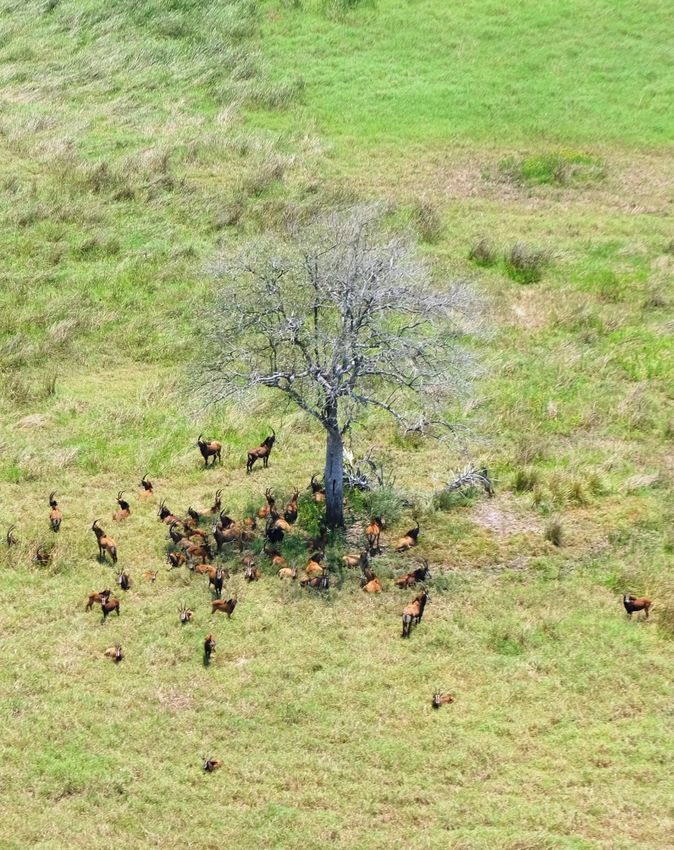
Table of contents
                Summary                                           3
                1. Survey methodology                             6
                        1.1. Flight observations and recording    6
                        1.2. Data handling                        7
                2. Results                                        8
                        2.1. Survey statistics                    8
                        2.2. Animal numbers recorded              11
                        2.3. Spatial distribution patterns        12
                        2.4. Wildlife biomass                     21
                        2.5. Additional species records           22
                        2.6. Illegal activities                   23
                3. Discussion                                     24
                        3.1. Context with regard to the drought   24
                        3.2. Side-by-side comparison with 2014    26
                4. Conclusion                                     29
                5. References                                     30
                6. Acknowledgements                               31

                                                                       2
Summary
                                                                                 Table 1: total number of herbivores counted in 2016
                                                                                   in the count block and additional sample lines.

• An aerial wildlife count of the Parque Nacional da Gorongosa was
                                                                                                                 Total number
  conducted between 18 and 31 October 2016.                                                      Species
                                                                                                                   counted

• The focus was on the Rift Valley in the southern and central sector of                 Blue wildebeest              363
  the park. A total of 184 500 hectares was fully covered by means of a                  Buffalo                      696
  helicopter. Systematic, parallel strips that were 500 m wide were                      Bushbuck                    2 062
  assessed. All large mammals observed were counted. All data, including                 Bushpig                      115
  geographical positions, were directly entered into a custom-made                       Common reedbuck            10 609
  census programme. In addition to this count block, a distance of
                                                                                         Duiker grey                   61
  respectively 100 and 125 km of transect lines were flown on the
                                                                                         Duiker red                    22
  western and eastern side of the core count area. This represents an
                                                                                         Eland                        118
  additional coverage of 11 250 ha. Total coverage through the central
                                                                                         Elephant*                    567
  counting block and these additional transect lines is 51.6% of the Park.
                                                                                         Hartebeest                   569

• A total of 78 627 herbivores of 19 species were counted (Table 1).                     Hippo                        440
  These are actual counts, not estimates. This represents the absolute                   Impala                      4 721
  minimum number of large animals that occur in the park.                                Kudu                        1 491
                                                                                         Nyala                       1 320
• Still more animals occur outside of the areas that were not counted.                   Oribi                       3 896
  However, the counting block represents the area with the best habitat                  Sable                        863
  and the highest known densities of wildlife as clearly illustrated by the              Warthog                     5 400
  much lower density and diversity of animals recorded along the sample                  Waterbuck**                45 280
  lines to the east and west.                                                            Zebra***                      34
                                                                                                                    78 627
                                                                              * 4 elephant added based on satellite collar data
                                                                              ** A total of 207 waterbuck were removed through live capture prior
                                                                                to the count and not included in this tally
                                                                              ** 15 held in the Sanctuary.                                     3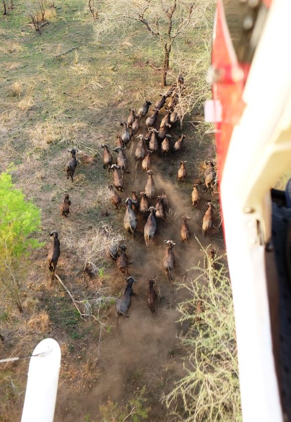
Summary - continued
• The previous two years have been very dry, in particular
over the months of January and February. These dry
conditions appear to have had a significant negative Table 2: side-by-side comparison between the numbers of animals in the
impact on several species (see page 5). same counting block surveyed in 2014 and 2016.
• The waterbuck have continued to increase and now 2016 as % of
number over 45 000 (Table 1). This represents a year-on- Species 2014 2016
2014
year increase of less than 15%. This is lower than Blue wildebeest 361 363 100.6
previous annual increment rates. This either reflects a Buffalo 670 696 103.9
slowing down of the population as it nears ecological Bushbuck 2 277 2 022 88.8
carrying capacity and/or it reflects the effects of the Bushpig 167 108 64.7
drought years on calf survival. Common reedbuck 11 871 10 451 88.0
Duiker grey 61 49 80.3
• Impala, kudu and nyala have increased substantially Duiker red 26 21 80.8
since 2014. Being predominantly browsers they are Eland 105 94 89.5
generally less affected by drought conditions. Elephant 535 567 106.0
Hartebeest 613 562 91.7
Hippo 436 440 100.9
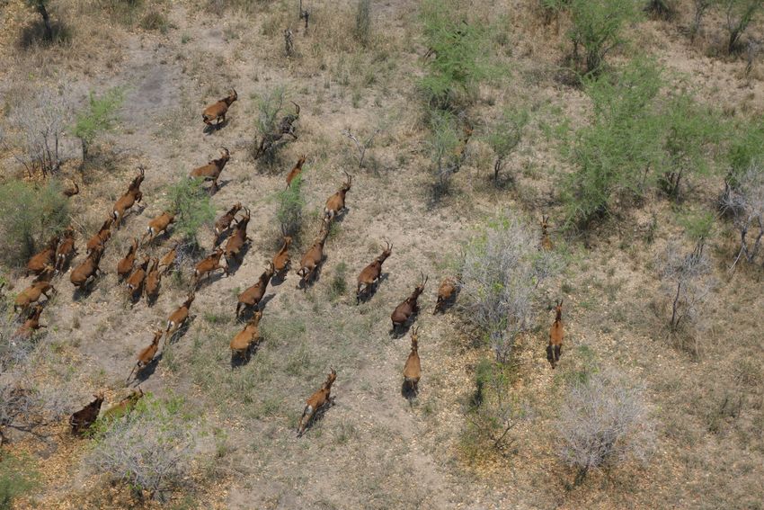
• The sable population now number over 800 in the
Impala 2 727 4 705 172.5
central part of the Park with several good herds being
Kudu 1 200 1 466 122.2
found in the miombo areas in the east. Nyala 945 1 299 137.5
Oribi 4 485 3 884 86.6
• Elephant and buffalo numbers are up despite the Sable 757 810 107.0
drought conditions. The latter grew with decreased or Warthog 9 086 5 383 59.2
less than expected increments. In the South African Waterbuck 34 482 44 948 130.4
lowveld, calving percentages have been extremely low Zebra 33 34 103.0
due to the prolonged drought conditions. TOTAL 70 837 77 902 110.0
• Blue wildebeest have remained stagnant, a concern that
was already identified in 2014.
4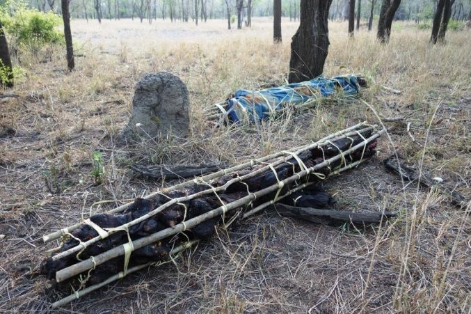
Summary - continued
• A group of smaller species including bushbuck, bushpig, common reedbuck,
  oribi and warthog have been substantially affected by the drought. These are
  mostly selective feeders requiring higher quality feed which may be reduced
  due to drought. Warthog in particular have declined in numbers. The latter
  species is typically the first to suffer from drought, but can also recover very
  quickly when conditions become favourable again.

• It has been noticeable how species such as buffalo have increased their range
  through the Park. Buffalo were observed for the first time as far north as
  Mucodza marsh, a distance of 54 km from their furthest south-eastern
  occurrence in the Park.

• Overall, a lower incidence of illegal activities was noted during the count.
  Whereas in 2014 a total of 4 freshly snared animals were encountered, only one
  (waterbuck) was observed during the 2016 count. Only one group of poachers
  was seen as against two groups observed in 2014. This decrease in the observed
  illegal activities would seem to reflect the good progress made in the
  recruitment and training of law enforcement personnel as well as in the
  improved tactics of deployment and organisation.

• Overall, the Park has weathered well the preceding drought years and the
  increased pressures of illegal hunting in a time of political turbulence. The
  recovery of the wildlife is progressing well.

• The 2016 count has re-affirmed the importance of these regular surveys. The
  aerial wildlife count using a helicopter is one of the most important and critical
  tools to evaluate the status of the recovery and the effectiveness of park
  management. It will be critically important to continue with regular counts.

                                                                                       5
1. Survey methodology
1.1. Flight observations and recording

The specific technique used was as follows:

  •    4-seat Bell Jet Ranger helicopter with the pilot in the right front seat, data
       capture / observer in the left front seat and two observers in the back;
  •    For the sake of maximum visibility, all doors of the helicopter are removed
       during the actual count;
  •    Parallel strips of 500 m width are flown. This means that observers look for
       wildlife in a strip of 250 m wide on each side of the helicopter. Marker bars
       indicate the strip width to avoid looking too far from the helicopter;
  •    The helicopter is maintained at a constant height of 50 to 55 m (160 feet)
       above the ground. Airspeed is maintained at around 96 km/h (60 knots).
       When a large herd is observed (e.g. impala) the pilot circles around to enable
       an accurate count;
  •    All animals are individually counted. The presence of baboon troops was
       recorded but the number of individual baboons is not enumerated;
  •    A separate flight was made from the middle Vunduzi River downstream to the
       confluence of the Urema-Pungue rivers to focus on crocodiles and hippo in
       the river and Lake system ;
  •    A GPS-based system (Global Positioning System) is used for accurate
       navigation. A grid is generated on a notebook computer that is linked to the
       helicopter’s GPS. Every 2 seconds a flight co-ordinate is downloaded onto the
       hard disc. When a sighting is made the position together with the species code
       and number is logged. The flight path and the observations are visible on
       screen. This enables the pilot to keep the helicopter on the pre-determined
       line and avoids the risk of areas not being covered or being covered twice. The
       position of the animals that have already been spotted is displayed on screen
       which assists in preventing double counting (Fig. 1);
  •    The observers in the back wear yellow goggles that reduce shadows and
       enhance contrast for better visibility and detection of the animals;
  •    Sessions lasting about two to three hours are flown. A short break is taken            Fig. 1: Example of actual flight lines and
       every hour to relieve observer fatigue. Two 3-hour or three 2-hour sessions       observations during the 2016 aerial wildlife count.
       can be flown in a single day depending on temperature and visibility.                                                              6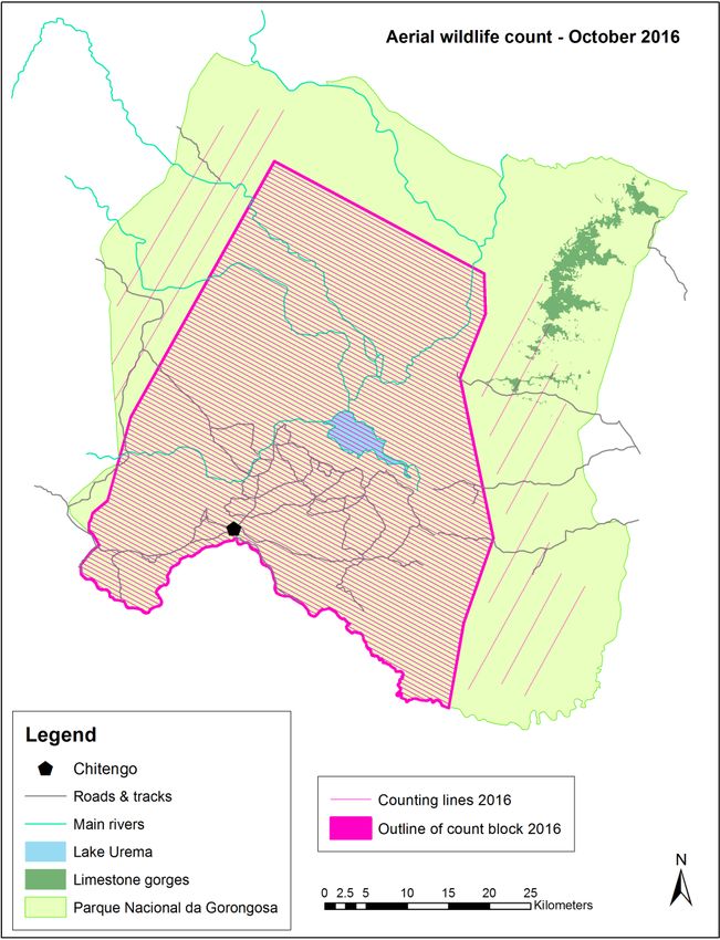
1.2. Data handling

Following their on-board capture, the data were consolidated into an Excel spreadsheet and exported to an
Access database. The 2016 data were amalgamated with the data from previous counts to facilitate analysis
and general comparisons.

Each data point has the following information:
       • Unique ID number
       • Day
       • Time
       • Count day and count session
       • Latitude / Longitude
       • Transect line
       • Species
       • Number of animals.

The relational Access data base allows linking these individual observations with other species characteristics
such as the average weight for each species that can be used for the calculation of stocking rates. The count
data were also converted to shapefiles for use in ArcGis.

   Id        Date           Time    Count_day        Session    Latitude   Longitude Line2014            Species       Number
 41113    10/24/2016    08:20:00 AM     6              16      -18.88860   34.39680     61              Waterbuck        28
 41114    10/24/2016    08:20:21 AM     6              16      -18.88620   34.39570     61              Waterbuck        34
 41115    10/24/2016    08:20:24 AM     6              16      -18.88570   34.39520     61               Warthog         5
 41116    10/24/2016    08:20:26 AM     6              16      -18.88560   34.39500     61               Impala          1
 41117    10/24/2016    08:20:27 AM     6              16      -18.88550   34.39490     61              Bushbuck         3
 41118    10/24/2016    08:20:33 AM     6              16      -18.88490   34.39380     61              Waterbuck        2
 41119    10/24/2016    08:20:35 AM     6              16      -18.88470   34.39340     61              Waterbuck        26
 41120    10/24/2016    08:20:39 AM     6              16      -18.88440   34.39270     61           Common reedbuck     1
 41121    10/24/2016    08:20:41 AM     6              16      -18.88430   34.39240     61              Waterbuck        3

                                                                                                                                7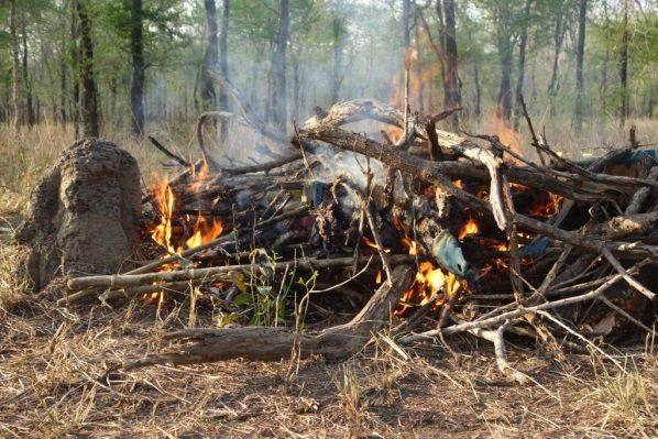
2. Results
2.1. Survey statistics

A count block of 184 500 hectares was fully covered by means of
a helicopter. In addition to this count block a distance of 100 and
125 km of transect lines were flown on the western and eastern
side of the count block respectively (Fig. 2). Total coverage
through the central counting block and the additional transect
lines in the east and west was 51.6% of the Park.

The total flying time for the survey was 79 hours. The average
area covered per flying hour was 2 330 hectares. This would vary
from day to day depending on distance from the base (longer or
shorter ferry time), density of the animals and nature of the
vegetation cover and structure.

This was pilot Mike Pingo’s eight helicopter wildlife count of
Gorongosa. Observer Dr Mike Peel from the Agricultural
Research Council is very experienced with wildlife counts in
South Africa. This was his third survey of Gorongosa. This was
also the third count of Gorongosa for data recorder Dr Marc
Stalmans. The remaining observer seat was mainly occupied by
Lukas Manaka (a very experienced counter from the Agricultural
Research Council).

Flying and counting conditions varied with some very hot days
being experienced (see Table 3). The counting sessions were
adjusted in order to avoid the hottest time of the day when
animals would tend to remain under the shade which made their
detection more difficult.                                             Fig. 2: Count block and additional sample lines
                                                                         covered by the 2016 aerial wildlife count.
                                                                                                                        8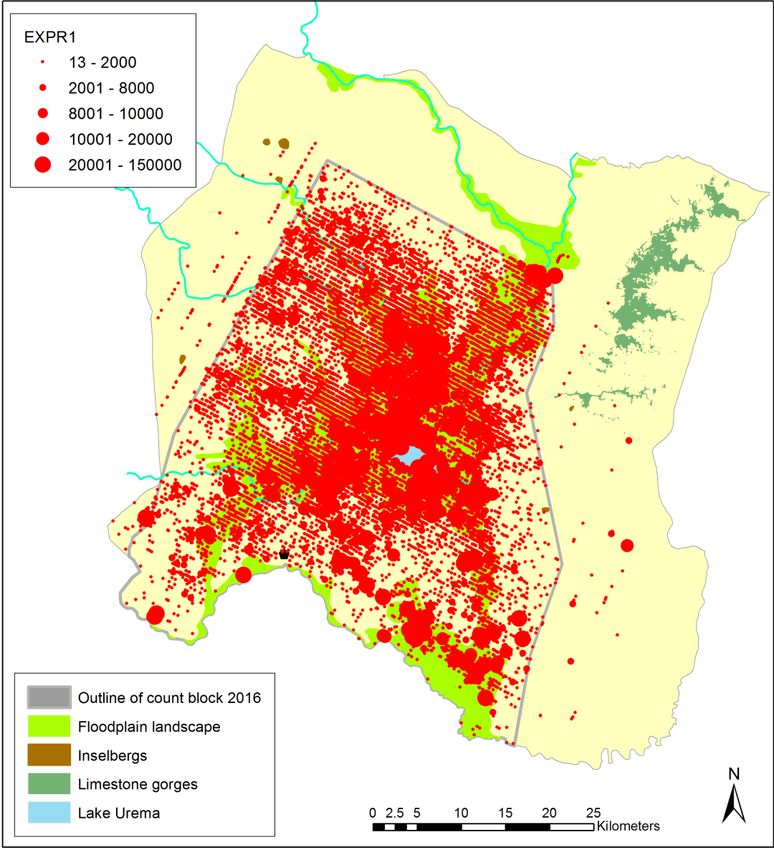
Table 3: Counting conditions during the 2016 aerial wildlife survey.

                                                                       9
Table 3 (continued): Counting conditions during the 2016 aerial wildlife survey.

                                                                                   10
Table 4: total number of herbivores
counted in 2016 in the count block
and additional sample lines.
Total number
Species
counted
2.2. Animal numbers recorded
Blue wildebeest 363
A total of 78 627 herbivores of 19 species were counted (Table 4). These are actual Buffalo 696
counts, not estimates. This represents the absolute minimum number of large Bushbuck 2 062
animals that occur in the park given that only 51.6% of the Park was counted. Bushpig 115
Common reedbuck 10 609
These records were amalgamated in the database together with the data from the Duiker grey 61
previous counts. The 2016 count generated 17 432 individual observations. At
Duiker red 22
present, the database holds 52 324 individual observations from 14 wildlife counts
Eland 118
since 1969.
Elephant* 567
Hartebeest 569
More animals still occur outside the block that was counted in 2014/2016, but no
Hippo 440
estimates were made. However, the count block represents the area with the best
habitat and the highest known densities of wildlife and is therefore likely to hold the Impala 4 721
bulk of most species as clearly illustrated by the much lower density and diversity of Kudu 1 491
animals recorded along the sample lines to the east and west (see section 3.2.). Nyala 1 320
Oribi 3 896
Sable 863
Warthog 5 400
Waterbuck** 45 280
Zebra*** 34
* 4 elephant added based on satellite collar data 78 627
** A total of 207 waterbuck were removed through live capture prior
to the count and not included in this tally
** 15 held in the Sanctuary. 112.3. Spatial distribution patterns
The distribution of the different
species across the count block
indicates a general preference for the
floodplain area1 and along the
perennial rivers such as Vunduzi,
Mucombeze and Urema Rivers. (Fig.
3).
Certain species are strongly associated
with the floodplain (e.g. waterbuck
and common reedbuck – Fig. 4 & 5),
others with the floodplain-woodland
interface (elephant and buffalo Fig. 6
& 7), and others still with the
woodlands (sable antelope,
Lichtenstein hartebeest, kudu, nyala
and impala – Fig. 8 to 12). The
distribution of wildebeest, zebra,
warthog and oribi is illustrated in Fig.
13 to 16. Hippo and crocodile are, as
expected, strongly associated with
Lake Urema and the perennial rivers
and pans (Fig. 17 & 18).
1 Floodplain landscape as defined by
Stalmans & Beilfuss (2008) Fig. 3: Spatial distribution of all observations during the 2016 aerial wildlife count.
12Fig. 4: Spatial distribution of waterbuck during the 2016 Fig. 5: Spatial distribution of common reedbuck during the
aerial wildlife count. 2016 aerial wildlife count.
13Fig. 6: Spatial distribution of elephant during the 2016 Fig. 7: Spatial distribution of buffalo during the 2016 aerial
aerial wildlife count. wildlife count.
14Fig. 8: Spatial distribution of sable antelope during the
2016 aerial wildlife count.
15Fig. 9: Spatial distribution of Lichtenstein hartebeest during Fig. 10: Spatial distribution of kudu during the 2016 aerial
the 2016 aerial wildlife count. wildlife count.
16Fig. 11: Spatial distribution of nyala during the 2016 aerial Fig. 12: Spatial distribution of impala during the 2016 aerial
wildlife count. wildlife count.
1715 in Sanctuary
Fig. 13: Spatial distribution of blue wildebeest during the Fig. 14: Spatial distribution of zebra during the 2016 aerial
2016 aerial wildlife count. wildlife count.
18Fig. 15: Spatial distribution of oribi during the 2016 aerial Fig. 16: Spatial distribution of warthog during the 2016
wildlife count. aerial wildlife count.
19Fig. 17: Spatial distribution of hippo during the 2016 aerial Fig. 18: Spatial distribution of crocodile during the 2016
wildlife count. aerial wildlife count.
202.4. Wildlife biomass
Biomass (kg)
The distribution of animal weight is plotted across the
landscape (Fig. 19). The highest animal biomass is
found in the floodplain around and north of Lake
Urema.
This translates to an average of 8 027 kg of biomass per
km2 which equates the conservative carrying capacity
of 8 000 kg per km2 calculated by Stalmans (2006) and
Stalmans & Beilfuss (2008). This is 16% up from the
average stocking of 6 913 kg per km2 calculated
following the 2014 count.
Fig. 19: Wildlife biomass across the landscape.
212.5. Additional species records
The presence of Crowned cranes, Saddle-bill storks and
Ground hornbills were recorded during the aerial survey.
These large birds are generally under some pressure in
southern Africa. A total of respectively 182 Ground hornbills,
119 Grey Crowned Cranes and 43 Saddle-bill storks were
observed.
A total of 225 baboon troops were recorded. This
information will be useful to the ongoing primatology
research project.
Although not a good tool to census lions, the helicopter count
did yield records of lions not yet know to the Lion Project.
Two young cubs were observed for the first time whilst one
adult lioness is likely also new.
A total of 9 active nests of White-headed vultures , 1 nest of Chitengo
Hooded vulture and 7 nests of White-backed vultures were
GPS’ed (Fig. 20). All three of these species are listed as
Critically Endangered.
Two Pel’s fishing owls were observed along the Vunduzi
River.
Lastly, a total of 86 active nests of Marabou storks were
GPS’ed. There is apparently only one other breeding locality
Fig. 20: Distribution of nests of vultures and of marabou
of this species known in Mozambique. storks observed during the 2016 aerial wildlife survey.
222.6. Illegal activities
During the count, signs of illegal activities
were recorded.
Overall, a lower incidence of illegal activities
were noted during this count. Whereas in
2014 a total of 4 freshly snared animals were
encountered, only one (waterbuck) was
observed during the 2016 count. It was
released from the snare but its ultimate fate
is unknown.
Only one group of poachers was seen as
against two groups observed in 2014. The
poachers fled and left behind two bundles of
smoked bushmeat. As it was in a remote
area, which precluded transporting the meat
back to Chitengo, these bundles were
incinerated (Fig. 22).
This decrease in the observed illegal
activities would seem to reflect the good
progress made in the recruitment and
training of law enforcement personnel as
well as in the improved tactics of
deployment and organisation.
Fig. 21: Intercepted bundles of smoked bushmeat that
were subsequently incinerated.
233. Discussion
3.1. Context with regard to the drought
Much of southern Africa has been in the grip of a profound mm rainfall
drought over the last 2 years. Gorongosa has not been an 1400
exception. The critical period for vegetation growth,
calving and calf survival extends from October till the end 1200
of February.
1000
The total rainfall received during the past two growing
seasons has been dramatically lower than that measured 800
the two years before (Fig. 22). During October 2014-2015
the rainfall was only 51% of that measured for the same 600
period in 2013-2014. In 2015-2016, the figure was even
lower with only 26% of the equivalent amount received in 400
2013-2014.
200
The low rainfall has resulted in a generally much reduced
grass production (Fig. 23). These dry conditions with 0
reduced availability of grazing can have a significant 2012-2013 2013-2014 2014-2015 2015-2016
negative impact on several wildlife species. Period October - February
Fig. 22: Rainfall received for the period October till
February over the past 4 years (note that these are
not annual totals, but reflect the rainfall across the
critical calving season).
24Note: generally reduced grass biomass in 2015, but especially in 2016
Fig. 23: Standing grass biomass (kg/ha) in the Rift Valley Alluvial Fan landscape
for a number of fixed monitoring transects (Peel 2016). 253.2. Side-by-side comparison with 2014
The 2016 results are compared to those for Table 5: side-by-side comparison between the numbers of animals in the
2014 for the same counting block (Table 5). same counting block surveyed in 2014 and 2016
Overall, the number of herbivores rose with
10% or more than 7 000 animals. 2016 as % of
Species 2014 2016
2014
The results are now discussed on a species- Blue wildebeest 361 363 100.6
by-species basis. Buffalo 670 696 103.9
Bushbuck 2 277 2 022 88.8
Bushpig 167 108 64.7
Common reedbuck 11 871 10 451 88.0
Duiker grey 61 49 80.3
Duiker red 26 21 80.8
Eland 105 94 89.5
Elephant 535 567 106.0
Hartebeest 613 562 91.7
Hippo 436 440 100.9
Impala 2 727 4 705 172.5
Kudu 1 200 1 466 122.2
Nyala 945 1 299 137.5
Oribi 4 485 3 884 86.6
Sable 757 810 107.0
Warthog 9 086 5 383 59.2
Waterbuck 34 482 44 948 130.4
Zebra 33 34 103.0
TOTAL 70 837 77 902 110.0
26• The waterbuck have continued to increase in numbers to • Impala, kudu and nyala have increased substantially since
over 45 000 (Table 1). This represents a year-on-year 2014. Being predominantly browsers they are generally
increase of less than 15%. This is lower than previous annual less affected by drought conditions.
increment rates. This either reflects a slowing down of the
population as it nears ecological carrying capacity and/or it • The sable population now number over 800 in the central
reflects the effects of the drought years on calf survival. part of the Park with several good herds being found in the
miombo areas in the east and west.
Anecdotally, during the capture of waterbuck earlier in
October for relocation to Zinave National Park and Maputo
• Elephant and buffalo numbers are up despite the drought
Special Reserve, it was observed that the waterbuck in the
conditions.
woodlands appeared to be in better physical condition than
those on the floodplain. At the time of the count, the
• Blue wildebeest have remained stagnant, a concern that
proportion of the waterbuck population found inside the
was already identified in 2014.
woodlands has increased substantially since 2014 (Fig. 24).
This probably reflects the higher availability of resources
• A group of smaller species including bushbuck, bushpig,
found at present within the woodlands.
common reedbuck, oribi and warthog have been
90.0 substantially affected by the drought. These are selective
80.0 feeders requiring higher quality feed which may be
reduced due to drought. Warthog in particular have
70.0
declined in numbers. This species is typically the first to
60.0
suffer from drought, but can also recover very quickly
50.0 when conditions become favourable again
%
40.0
30.0 • It has been noticeable how species such as buffalo have
increased their range through the Park. Buffalo were
20.0
observed for the first time as far north as Mucodza marsh,
10.0 a distance of 54 km from their furthest south-eastern
0.0 occurrence in the Park (Fig. 7).
2014 2016
Floodplain habitat Woodland habitat
Fig. 24: Shift in habitat occupation by waterbuck from 2014 to 2016. 27• Still more animals occur outside of the areas of the central
counting block. However, densities of most species are much
lower to the east and west as measured through the
Table 6: Wildlife densities (as animals per km2) across the western,
(limited) sampling lines flown (Table 6).
central and eastern parts of Gorongosa National Park
The difference is often an order of magnitude or more in Western Central Eastern
wildlife densities. This is a reflection of the more infertile Species
sample lines countblock sample lines
habitat on the eastern and western rim of the Rift Valley.
Bushbuck 0.32 1.10 0.19
However it more than likely also reflects the still incomplete
Common reedbuck 0.58 5.66 0.08
nature of the restoration and the expected higher pressure
Duiker grey 0.10 0.03 0.06
from illegal hunting closer to the Park boundaries.
Impala 0.14 2.55 0.14
Kudu 0.26 0.79 0.00
Sable antelope do well in the eastern miombo. A total of 53
Nyala 0.10 0.70 0.21
sable in 5 herds were observed along the few sample lines
Warthog 0.20 2.92 0.35
flown. Sable tend to do well in a low-competition
Waterbuck 1.48 24.36 0.00
environment. to A herd of 24 eland were also observed in
the east.
Interestingly enough, no waterbuck were observed at all to
the east of the counting block. A low density of waterbuck
was recorded in the west.
Grey duikers are occurring at higher densities in the west
and east which conforms with their known habitat
preferences.
284. Conclusion
In conclusion, the 2016 aerial wildlife count
was successful.
This was the second block count that
covered 100% of the central, and most
important, part of the Gorongosa National
Park.
Overall, the Park has weathered well the
preceding drought years and the increased
pressures of illegal hunting in a time of
political turbulence. The recovery of the
wildlife is progressing well.
The aerial wildlife count using a helicopter is
one of the most important and critical tools
to evaluate the status of the recovery and
the effectiveness of park management. It
will be critically important to continue with
regular counts. The aerial wildlife count is a
vital M&E tool for the Park.
295. References
Peel M. 2016. Ecological Monitoring: Parque Nacional Da
Gorongosa, Moҫambique. Unpublished report by the Agricultural
Research Council to the Gorongosa Restoration Project.
Stalmans M. 2006. Vegetation and carrying capacity of the
‘Santuario’, Parque Nacional da Gorongosa, Moçambique.
Unpublished report by International Conservation Services to the
Carr Foundation and the Ministry of Tourism.
Stalmans M. & Beilfuss R. 2008. Landscapes of the Gorongosa
National Park. Unpublished report to the Gorongosa Restoration
Project.
Stalmans M., Peel M. & Massad T. 2014. Aerial wildlife count of the
Parque Nacional da Gorongosa, Mozambique, October 2014 -
Approach, results and discussion. Unpublished report to the
Gorongosa Restoration Project.
Tinley. K.L. 1977. Framework of the Gorongosa Ecosystem. PhD
thesis. University of Pretoria.
306. Acknowledgements
The helicopter survey would not have been possible
without the input and assistance of many people. The
following are acknowledged:
• The GRP and its partners, in particular USAID, for
the funding of the survey;
• Park and government authorities for the
necessary clearances;
• Helicopter pilot Mike Pingo for his highly
professional and experienced flying of the survey
including advice on the best counting conditions
and approaches;
• Dr Mike Peel of the Agricultural Research Council
for his counting role and inputs based on many
years of similar wildlife counts in southern
Africa;
• All of the other observers for their professional
approach to the counting job, namely Lukas
Manaka of the Agricultural Research Council,
Gregory Pingo and Jason Denlinger ;
• Mike Marchington and his team for the logistical
support offered at Chitengo in particular with
the refuelling.
31You can also read