Amelia Earhart and the Nikumaroro Bones A 1941 Analysis versus Modern Quantitative Techniques - University of Florida Press ...
←
→
Page content transcription
If your browser does not render page correctly, please read the page content below
Forensic Anthropology Vol. 1, No. 2: 83–98
DOI 10.5744/fa.2018.0009
RESEARCH ARTICLE
Amelia Earhart and the Nikumaroro Bones
A 1941 Analysis versus Modern Quantitative Techniques
Richard L. Jantza*
ABSTRACT: The unknown fate of Amelia Earhart continues to fascinate. One of the most tantalizing clues involves skeletal remains
found on Nikumaroro Island in 1940. Some have summarily dismissed these bones as the remains of Amelia Earhart because they were
assessed as male by Dr. D. W. Hoodless, principal of the Central Medical School, Fiji, in 1940. The most recent such dismissal is that of
Cross and Wright (2015), who argue that Hoodless’s methods were sound and therefore his sex estimate was likely correct.
This paper addresses two issues: (1) it evaluates Hoodless’s methods and Cross and Wright’s support of them, and (2) it compares the
Nikumaroro bones with what we can learn about Amelia Earhart’s bone lengths.
When Hoodless conducted his analysis, forensic osteology was not yet a well-developed discipline. Evaluating his methods with refer-
ence to modern data and methods suggests that they were inadequate to his task; this is particularly the case with his sexing method. There-
fore his sex assessment of the Nikumaroro bones cannot be assumed to be correct.
To address the question of whether the Nikumaroro bones match estimates of Amelia Earhart’s bone lengths, I compare Earhart’s bone
lengths with the Nikumaroro bones using Mahalanobis distance. This analysis reveals that Earhart is more similar to the Nikumaroro bones
than 99% of individuals in a large reference sample. This strongly supports the conclusion that the Nikumaroro bones belonged to Amelia
Earhart.
KEYWORDS: forensic anthropology, Amelia Earhart, human identification, multivariate
Introduction including a humerus, radius, tibia, fibula, and both femora.
The bones were apparently complete, but they had experi-
The fate of Amelia Earhart continues to captivate public and enced some taphonomic modification. Also found were part
scientific attention. Several hypotheses, some more credible of a shoe, judged to have been a woman’s; a sextant box,
than others, have been advanced about what may have hap- designed to carry a Brandis Navy Surveying Sextant manu-
pened to her and her navigator, Fred Noonan, on their ill-fated factured circa 1918; and a Benedictine bottle. There was sus-
attempt to fly around the world. One intriguing component picion at the time that the bones could be the remains of
of the Earhart mystery involves whether bones found on Amelia Earhart.1
Nikumaroro Island in 1940 could be her remains, suggest- Although the bones themselves have been lost (cf. King
ing she died as a castaway on this remote island. This paper 1999), Burns et al. (1998) analyzed measurements taken in
will subject this idea to scientific analysis to determine 1941 by Dr. D. W. Hoodless, principal of the Central Medi-
whether the evidence supports the conclusion that the bones cal School, Fiji. They concluded that the bones were more
belong to Earhart or whether she can be excluded. likely those of a female of European ancestry and between
The bones in question were found in 1940 when a work- 5'6" and 5'8" tall, a biological profile entirely consistent with
ing party brought to Nikumaroro for the Phoenix Island Set- Amelia Earhart. These conclusions conflicted with those of
tlement Scheme found and buried a human skull. Upon Hoodless, who had assessed the remains as belonging to a
hearing of the discovery, the officer in charge of the settle- middle-aged stocky male about 5'5.5" in height.2 The Burns
ment scheme, Gerald Gallagher, ordered a more thorough et al. report prompted a rebuttal by Cross and Wright (2015),
search of the area. The search resulted in additional bones, who put forth two general arguments: (1) that Hoodless was
qualified to conduct a forensic anthropological examination
a
Department of Anthropology, University of Tennessee, Knoxville, of the remains and therefore was most likely correct in his
TN 37996, USA assessment, particularly the sex assessment, so the bones
*Correspondence to: Richard L. Jantz, Department of Anthropology,
505 Strong Hall, University of Tennessee, Knoxville, TN 37996, USA
E-mail: rjantz@utk.edu 1. For a full account of the discovery, see https://tighar.org/Publications
/TTracks/13_1/tarawa.html.
Received 16 August 2017; Revised 14 October 2017; Accepted 27 2. For Hoodless’s notes on his analysis, see https://tighar.org/Projects
November 2017 /Earhart/Archives/Documents/Bones_Chronology4.html.
© 2018 University of Florida Press84 Amelia Earhart and Nikumaroro Bones
were unlikely to have been Earhart’s remains; and (2) that Earhart’s clothing held in the George Palmer Putnam Col-
Earhart’s physique was extremely linear and gracile, and lection of Amelia Earhart Papers held at Purdue University.
therefore inconsistent with Hoodless’s assessment of the These articles of clothing were kindly made available for
remains as those of a stocky male. Both of these arguments measurement by Purdue University archivist Sammie Mor-
turn on the accuracy of Hoodless’s assessment. riss. Historic clothing seamstress Paula Guernsey took the
Cross and Wright (2015:53) acknowledge that Hoodless measurements. The measurements used in this report are
was “obviously not trained as a modern forensic anthropol- inseam length and waist circumference taken from a pair of
ogist,” but they assert that “his background indicates he was Earhart’s trousers.
perfectly competent to assess sex, age, body type, and ances- It has been shown that measurements have considerable
try of a human skeleton.” Implicit in this argument is that potential to individualize. Sassouni (1960) achieved 100 per-
Hoodless’s background as a teacher of anatomy and his train- cent matching of premortem cranial radiographs to post-
ing in medical practice qualified him to assess biological mortem candidates using eight cranial measurements. In an
profile with little probability of error. On the central ques- analogous situation, pair matching has proved effective in
tion of sex, Cross and Wright (2015) do not evaluate the meth- reassociating commingled remains (Lynch et al. 2017). The
ods Hoodless used but accept them as valid and still in use fit of the Nikumaroro bones to Amelia Earhart was assessed
today. There is also considerable information not considered using Mahalanobis distance (D) and considered in relation
by Cross and Wright (2015) that bears on the question of to all other individuals in the database. Acquisition of Ear-
Earhart’s body size and shape, how these relate to what we hart’s bone lengths is described further on.
know about the bones, and Hoodless’s interpretation of them. Other statistical methods used are well known and require
This paper consists of two parts. The first part examines little description. I introduce them briefly where they are used
the methods Hoodless used and which were so vigorously and describe their applicability to the question at hand.
defended by Cross and Wright (2015). It subjects the appli-
cation of these methods to quantitative verification, and
wherever possible includes new analyses. It examines the Hoodless’s Methods and the State of the
state of forensic anthropology in 1941 to provide the context Art in 1941
in which Hoodless worked. The second part examines Ame-
lia Earhart’s body size and shape to determine whether they There are both general and specific reasons to question Hood-
fit the meager evidence at hand and whether there may be rea- less’s analysis. These do not relate to his competence as
sons to believe that Hoodless was deceived by what he saw much as they do to the state of forensic anthropology at the
before him. These analyses result in a refined conclusion as time. Forensic anthropology was not well developed in the
to whether the remains examined by Hoodless were likely early 20th century. There are many examples of erroneous
those of Amelia Earhart. assessments by anthropologists of the period. E. A. Hooton,
one of the most prominent and influential biological anthro-
pologists of the early to mid-20th century, had considerable
Materials and Methods difficulty sexing the skeletons from Pecos Pueblo, ending up
with a sex ratio favoring males (Hooton 1930). Weisensee and
Metric data from the Nikumaroro bones are limited to seven Jantz (2010) and Tague (2010) have reexamined the Pecos col-
measurements, four of the skull (maximum cranial length, lection and concluded that Hooton sexed too many females
maximum cranial breadth, orbital height, and orbital breadth) as males, likely because he gave the skull more weight than
and three long bone measurements (length of the humerus, the pelvis in his sex assessments.
radius, and tibia; see Burns et al. 1998 for measurements). I G. K. Neumann is known for establishing a typological
use data from the Forensic Anthropology Data Bank (FDB), framework for Native American remains (Neumann 1952).
Trotter’s U.S. military data (see Jantz & Meadows Jantz 2017 In so doing he examined hundreds of crania from different
for full description of data), and literature sources to evalu- parts of the United States. Yet when confronted with a cra-
ate quantitatively both Hoodless’s methods and Cross and nium from Jamestown, clearly of African ancestry, he mis-
Wright’s (2015) claims about the former’s effectiveness. I identified it as Native American (Neumann 1958), presumably
reassess cranial affinities using Fordisc 3.1 (Jantz & Ousley because the archaeologist who excavated it thought it to be
2005) with realistic assumptions about who could have been Native American (see Cotter 1958:24).
on Nikumaroro Island during the relevant time period. Ear- Given the state of the art at the time, why should we sup-
hart’s bone lengths were estimated using photographic evi- pose that Hoodless, who as far as we know had no formal
dence and regression analysis. training in forensic anthropology and had not examined large
Additional information concerning Amelia Earhart’s numbers of skeletons (if any at all), was ahead of his time in
body dimensions came to light in 2017 through study of the forensic analysis of skeletal remains? It is unreasonableJantz 85
to view Hoodless, or any analyst of that time or this, as TABLE 1—Comparison of Pearson’s stature with more recent
capable of making such assessments without error. Modern estimation equations from 19th century, Trotter’s WW2 (males only),
and modern forensic statures from Fordisc 3.1 (Jantz & Ousley 2005).
forensic anthropologists with training and experience still
make errors, and the need to have estimates of error rates is Humerus Radius Tibia Combined
receiving increased attention in view of the Daubert ruling.3 Equation Source (cm) (cm) (cm) (cm)
Cognitive bias (i.e., bias resulting from prior information) is Pearson males 164.4 166.1 167.1
especially problematic when making visual assessments Pearson females 160.7 163.1 162.3
19th males 168.6 170.8 172.7 170.8
(Nakhaeizadeh et al. 2014). We do not know whether cogni- 19th females 168.1 171.1 168.5 170.4
tive bias may have played a role in Hoodless’s evaluation, but Trotter’s WW2 170.7 172.1 170.1 170.4
20th Fstats males 172.4 172.4 170.9 171.4
the possibility cannot be ruled out. 20th Fstats females 168.2 169.0 166.3 167.9
We can agree that Hoodless may have done as well as
most analysts of the time could have done, but this does not
mean his analysis was correct. All we now have are the few yields a height of circa 161–163 cm (63–64 in.), seemingly a
measurements he gave in his report and his brief summary serious underestimate.
of the methods he used. It is important to extract as much as An examination of Pearson’s sample will clarify why his
possible from the information at hand. In doing so, I will equations are not appropriate for modern people. Pearson
show that Cross and Wright (2015) present Hoodless as more used Manouvrier’s French sample, consisting of only 50 indi-
unerring in forensic anthropology than most anthropologists viduals of each sex. These were individuals whose birth
of his time, and further that they have misinterpreted some years would likely have been early 19th century and who
of the other data available about Amelia Earhart. were substantially shorter than modern Americans or even
Americans of the late 19th century. Pearson used an estimate
Stature Estimation of 165 cm to calculate the intercept for his male equations.
This agrees well with Fogel’s (2004) values of 164.3 cm and
Hoodless estimated stature using Pearson’s (1899) formulae. 165.2 cm for French males reaching maturity in the first and
He cannot be faulted for this, because little else was avail- second quarter of the 19th century, respectively. French
able at the time. Cross and Wright (2015) argue that Pearson’s women were estimated by different methods to arrive at
formulae are still in use today. I am not aware of any con- a value of 152.3 cm. By contrast, American males born in
temporary forensic anthropologist that uses Pearson’s formu- the 1890s were 169.1 cm and in the first decade of the 1900s
lae. Recent forensic anthropology textbooks either mention were 170.0 cm (Floud et al. 2011), some 4–5 cm greater than
Pearson as important in developing the regression approach early-19th-century French. Floud et al. (2011) do not present
still in use today but omit his formulae, or do not mention data for females before 1910, but those born in that decade
him at all. Guharaj (2003) does include Pearson’s formulae, were 160.6, some 8 cm greater than the French value used
but, interestingly, includes the same erroneous constant for by Pearson.
the radius that Hoodless used. This suggests that neither Figure 1 shows an example, using the humerus, of the
Guharaj nor Hoodless consulted Pearson’s original paper. relationship between bone length and stature. It illustrates the
Their shared error must go back to a common source. nature of the differences between Pearson’s sample and Trot-
I have computed estimates from the more recent stature ter and Gleser’s (1952) 19th-century samples. The slopes are
estimation criteria contained in Fordisc 3.1 and compared approximately equal, but the 19th-century regression lines
them to Pearson’s (Table 1). Pearson’s equations consistently are elevated, yielding higher estimates for a given bone
underestimate height compared to modern criteria. Only one length.
of Pearson’s estimates exceeds the 20 more-modern estimates Parenthetically, it is curious that Hoodless characterized
in Table 1. Pearson’s male tibia estimate exceeds the 20th- the bones as possibly those of a “short, stocky muscular Euro-
century female forensic stature estimate. By any reasonable pean,” when his own height estimate places the individual
standard, the height of 65.5 inches (166.4 cm) presented by only slightly below the average for both American and Euro-
Hoodless and supported by Cross and Wright (2015) must be pean males born at the end of the 19th century and early in
considered an underestimate. If the bones actually belong to the 20th century.
a male, as Hoodless concluded, then the best estimate of
height is about 170 cm, or about 67 inches. If the bones belong Hoodless’s Sex Assessement
to a female, then about 169 cm, or 66.5 inches, is the most
reasonable estimate. Using Pearson’s equation for females Cross and Wright (2015) argue that sex is the Earhart dis-
qualifier, and indeed it could be, if firmly established. They
3. On the Daubert standard, see http://www.forensicsciencesimplified are at some pains to present Hoodless as possessing suffi-
.org/legal/daubert.html cient expertise to leave little doubt about his sex assessment.86 Amelia Earhart and Nikumaroro Bones
to its length as an example of this approach. Femur circum-
ference alone is dimorphic enough to qualify as a moder-
ately good sex estimator (DiBennardo & Taylor 1979; Black
1978), but I have been unable to locate published references
to use of the ratio of circumference to length as a dimorphic
trait to estimate sex. No reference was provided by Cross and
Wright (2015).
Whether the ratios Hoodless employed are dimorphic
enough to provide an indication of sex is subject to empiri-
cal verification. Table 2 shows discrimination statistics,
using Euro-American femur data from the FDB for the cir-
cumference ratio, circumference alone, and femur length
alone. Classification efficiency was assessed using an index
of discrimination defined by Maynard-Smith et al. (1961) as
(xm − xf )/(sdm + sdf ), the difference between sex means divided
by the sum of the standard deviations. The percentage of
correct classifications can be estimated by relating the index
to a cumulative normal distribution. This provides a close
approximation to empirical classification rates.
The best single variable is circumference, sexing around
FIG. 1—Comparison of Pearson’s regression lines (short dashes =
females, long dashes = males) with Trotter and Gleser’s 19th century
about 80% correctly. Femur length yields almost 78%. The
(dotted = females, solid = males). The lengths of the lines on the x axis sex difference in the ratio of circumference to length is highly
are set at ±2 standard deviations from their respective means. The significant, showing that males have a more robust midshaft
shorter lines associated with Pearson’s data show lower variance than females. But the accuracy of assessing sex this way is
compared to 19th-century Americans. The triangles are the position of
the Nikumaroro humerus. Note that the Nikumaroro point for Pearson
60%, only about 10% better than guessing. The ratio dilutes
females is close to the upper maximum, where estimation is more dimorphism, so it is almost 20% worse than circumference
unreliable, especially with small sample sizes. alone.
“Set” of the femora. Using the femur for sex estimation is
Hoodless’s self-reported criteria were (1) half subpubic now common (Spradley & Jantz 2011), but I have been unable
angle; (2) “set” of the femora; and (3) ratio of the long bone to find any reference to “set” of the femora, clarified by
circumferences to their lengths. Cross and Wright (2015) go Cross and Wright (2015) as the angulation to the pelvis. Pre-
on to say these features are still used today. I am unaware sumably it has something to do with angle of the femur neck
that “set” of the femora and ratio of circumferences to length and the distal condyles to the diaphysis. The angle of the
are used as a sexing criterion by forensic anthropologists distal condyles to the diaphysis was included in Dibenarrdo
practicing today. Evaluating these variables with data will and Taylor’s (1983) analysis of sex and ancestry variation of
demonstrate why they are not used. I will also show that the femur. For Euro-Americans of the Terry collection these
estimating sex from the half subpubic angle is by no means values were 79.8 and 78.1 for males and females, respectively.
foolproof. The standard deviations were 2.1 for both sexes. The sex dif-
ference is small and significant (t = 4.5, df = 128, p < 0.001),
Ratio of femur circumference to length. Although Hoodless but the overlap of the two distributions is too large to allow
apparently used the ratio of circumference to length of sev- reliable sexing. Estimating accuracy from the index of dis-
eral long bones, I will use the ratio of femur circumference crimination yields an expectation of about 65% correct. It is
TABLE 2—Sexing accuracy of circumference of the femur (C), length of the femur (L), and ratio of
circumference to length.
Females Males Discrimination Statistics
Index of Percent
Femur Variable Mean SD Mean SD F ratio Discrimination Correct
(C/L)*100 18.869 1.306 19.595 1.161 58.19 0.294 61.6
C 82.483 5.895 92.328 5.722 469.01 0.848 80.2
L 437.605 21.381 471.674 23.060 369.25 0.767 77.8Jantz 87
slightly better than the ratio of circumference to length, but
still only 15% better than guessing, not something that could
be used to reliably assess sex. The sex difference of 1.7°
would presumably be very difficult to appreciate via visual
assessment.
The angle of the femur neck to the diaphysis is no bet-
ter. Anderson and Trinkaus (1998) could not identify consis-
tent sex differences among world populations. In a sample of
modern Euro-Americans the sex difference was 1.9°, which
was not significant and would be difficult to appreciate by
visual inspection.
Half subpubic angle. The subpubic angle is defined as the
angle formed by the two ischio-pubic ramii with an apex at
the inferior junction of the pubic bones. This feature is unde-
niably a dimorphic feature, and in the hands of an experi-
enced forensic anthropologist it can yield high accuracy
rates, although not 100%. While it can be measured, in my
experience that is rarely done by forensic anthropologists. FIG. 2—Barchart of ordinal scores for the subpubic contour, which
The half subpubic angle requires assessing the angle from a forms one half of the subpubic angle. A substantial minority (20%) of
single innominate, presumably more difficult than assessing females (white bars) have scores that are either ambiguous (SC = 3) or
male (SC = 4 or 5). Data from Klales et al. (2012).
it when both are present. There are some issues that reduce
the certainty of Hoodless’s estimate. Especially important is
Hoodless’s description of the condition of the bones: “All Klales et al. (2012) have devised a systematic, five-stage
these bones are very weather-beaten and have been exposed ordinal scoring system for the Phenice traits, including the
to the open air for a considerable time. Except in one or two subpubic contour. Part of their sample was drawn from the
small areas all traces of muscular attachments and the various Hamann-Todd anatomical collection, which is a reasonable
ridges and prominences have been obliterated.” (W.P.H.C.:15) reference sample for the Nikumaroro bones. Figure 2 shows
Damage to the bones was most likely due to scavenging by the distribution of the Hamann-Todd sample on the five-stage
crabs, as originally observed by Gerald Gallagher, adminis- scores of Klales et al. (2012). The scores range from strongly
trator of the Phoenix Island settlement scheme, who also female (stage 1) to strongly male (stage 5). The graph shows
opined that the bones were from a female based on associa- that most females are stage 1 or 2, and most males are stage
tion with a women’s shoe sole.4 The fragile pubic bones 4 or 5. But there is a sizable minority of females (21% of the
would have been especially susceptible to damage. It is not female sample) in stage 3 or higher. Stage 3 is the antimode
beyond imagination that bone morphology was sufficiently between the two distributions and describes an ambiguous
modified to reduce ability to accurately assess the half sub- subpubic contour that could easily be called either male or
pubic angle. female. Klales (2016) has documented that the subpubic
Even without taphonomic change, sex estimates can vary contour has experienced secular change, the number of
widely. A method put forth by Phenice (1969) is commonly ambiguous females declining since 1940. These data suggest
accepted as reliable. The Phenice method uses three features that Hoodless could easily have been presented with mor-
of the pubic bone, including the subpubic contour. It should phology that he considered male, even though it may have
be noted that the subpubic contour does not entirely define been female.
the subpubic angle, but as Klales et al. (2012) note, the female
concavity results in a greater subpubic angle, which would Overall Assessment of Hoodless’s Sex Estimate
likely play a large role in visual assessment of the subpubic
angle. Klales et al. (2012) present the results of eight tests of Hoodless based his conclusion on three features, one of
the Phenice method. They range from 59% to 99% in sexing which—the ratio of circumference to length, as exemplified
accuracy. Of the eight tests presented, four sexed correctly by the femur—is not sufficiently dimorphic to provide use-
at less than 90%. These tests used all three of Phenice’s traits; ful information. The second feature, “set” of the femora, is
presumably the subpubic contour alone would perform worse also minimally informative. The subpubic angle, the most
than all three combined. reliable of Hoodless’s criteria, is also subject to considerable
variation, much of which was little understood in 1941. We
4. See https://tighar.org/wiki/Bones_found_on_Nikumaroro. do not know what weight Hoodless attached to each feature.88 Amelia Earhart and Nikumaroro Bones
He must have considered the two doubtful features to some If the problem is approached using only samples of pop-
degree, and perhaps given them weights equal to the subpu- ulations that might reasonably have been on the island,
bic angle. Otherwise he would not have mentioned them. somewhat more definitive results are obtained. Ancestries
Cross and Wright (2015) argue that Hoodless undoubt- other than European would include Micronesians and
edly made an overall assessment of the remains, including Polynesians. I use a Euro-American sample of the early 20th
the skull, but only reported the less detailed information century, a Micronesian sample (Guam), and a Polynesian
appropriate to his audience. How this overall assessment sample (Moriori), the last two from Howells’s data. Ideally
might have informed his decision is pure speculation. No one the Micronesian sample should come from the Eastern
knows what the skull or postcranial skeleton looked like, nor Micronesians, but data are limited. Pietrusewsky’s (1990)
what Hoodless used to arrive at his assessment of robustic- samples are small and limited to males, but they argue for a
ity. It is also worth noting that while demonstrating aware- basic continuity among Micronesians. The same is true for
ness of Pearson’s (1899) stature estimation paper, Hoodless Polynesians, so Guam and Moriori can be accepted as rea-
was either unaware of or chose not to mention Pearson and sonable representations of these two areas.
Bell’s (1919) paper—which provided valid sexing criteria for Table 3 shows Fordisc results for Euro-Americans and
the femur, such as the femur head diameter. The state of the Pacific Islanders, each with both sexes. The lowest Mahala-
art at the time, and the fact that Hoodless was not an experi- nobis distance and the highest posterior probability belong
enced forensic anthropologist, reduce the reliability of Hood- to early-20th-century Euro-American females. Because the
less’s sex estimate considerably below that accorded it by discriminating ability of four measurements is low, the skull
Cross and Wright (2015). The most prudent position con- cannot be excluded from any of the populations used, as
cerning sex of the Nikumaroro bones is to consider them shown by the typicality probabilities. The Typ R, the ranked
unknown. typicality probability column, provides some additional use-
ful information. Typ R is the ranking of each skull’s dis-
Hoodless’s Ancestry Estimate tance from the sample mean. A typicality probability of 1.0
would indicate that all the values are identical to the mean.
It is the case, as Cross and Wright (2015) have stated, that Euro-American females have the highest typicality probabil-
little convincing evidence concerning the ancestry of the ity. Only 6 crania of 90 are more typical than the Nikuma-
Nikumaroro bones can be gained from the four cranial mea- roro skull. Typicalities for all other groups are 0.65 or less.
surements Hoodless provided. However, this is not to say we Another avenue toward ancestry assessment could lie in
cannot get more evidence than offered by Hoodless, or by the long bone lengths, since different populations have differ-
Cross and Wright (2015). Hoodless’s assessment that the skel- ent long bone proportions. This can be approached quantita-
eton is not full Pacific Islander but could be a “short stocky, tively using distance statistics parallel to those used for the
muscular European or even a half-caste or a person of mixed cranial analysis. We do not have a database containing bone
European descent” (W.P.H.C.:15) may reflect assumptions lengths from different populations, but it is possible to use
that conflict with his own assessment of the two indices he published means as long as one has a covariance matrix. It has
computed—orbital and cranial—both of which indicated been shown that the long bone length covariance matrices from
European. Cross and Wright’s (2015) CRANID analysis is widely different populations are homogeneous (Holliday &
flawed because they included samples from all over the world, Ruff 2001). Therefore I use mean long bone lengths from
most of them including individuals from populations that had Hawaiian and Chomorro people as representative of Pacific
zero or near zero probability of having been on Nikumaroro. Islanders (Polynesia and Micronesia) (Ishida 1993), and 19th-
Konigsberg et al. (2009) have shown the importance of an century (Terry collection) and 20th-century Whites (FDB)
informative prior probability in ancestry estimation. If the from which the covariance matrix was obtained.
prior probability is zero, then the posterior probability must Figure 3 shows the distances plotted on the first two
also be zero. canonical axes obtained from humerus, tibia, and radius
TABLE 3—Fordisc 3.1 output for Nikumaroro skull, compared to Euro-Americans and Pacific Islanders.
Probabilities
Classified Distance
Group into from Posterior Typ F Typ Chi Typ R
E20F **E20F** 0.8 0.318 0.941 0.940 0.933 (7/90)
GUAMF 1.7 0.200 0.802 0.788 0.500 (15/28)
MORIF 1.7 0.199 0.795 0.786 0.654 (19/52)
GUAMM 2.3 0.146 0.691 0.673 0.581 (14/31)
E20M 3.3 0.092 0.523 0.514 0.624 (48/125)
MORIM 4.7 0.045 0.333 0.317 0.276 (43/58)Jantz 89
FIG. 3—Canonical plot of Euro-Americans, Hawaiians, and Chomorro from bone lengths. The Nikumaroro bones
were interpolated into the plot using distances from other groups. The first axis mainly reflects size and hence sex
differences. The second axis mainly reflects humerus and tibia lengths, low scores reflecting longer humeri and tibiae.
The Nikumaroro bones fall on the male side on CV1 and on the Euro-American side on CV2.
length. The first axis is mainly size and therefore reflects sex called a forensic stature, meaning that it comes from a doc-
differences. The second axis reflects mainly humerus and ument rather than being explicitly measured. The air com-
tibia lengths, low scores reflecting longer humeri and tibiae. merce regulations for 1928 state the following:
The Nikumaroro bones were interpolated into the plot using
the distances from each group as described by Gower (1972). An application for a pilot’s license must be filed, under
The Nikumaroro bones are most similar to White males. oath, with the Secretary of Commerce upon blanks fur-
They are most distant from Pacific Islanders, particularly nished for that purpose. An applicant for a pilot’s license,
Chomorro Micronesians. including a student’s pilot license, must appear for a
physical examination before a physician designated by
the Secretary of Commerce and pass such examination,
Amelia Earhart’s Height, Weight, Body Build, unless he is exempt under these regulations.
and Limb Lengths and Proportions
There appears to be no explicit requirement that height
I will now try to reconstruct what I can about Amelia Ear- must be measured. If it was measured, it could have been
hart’s, height, weight, body build, and limb lengths and pro- done either freestanding or standing against a wall. We have
portions. This will serve two purposes: (1) allow testing of no idea of the skill or attention to detail the examiner might
Cross and Wright’s (2015) assumption that she was extremely have brought to the task. Was Earhart properly positioned
linear and gracile, and (2) allow explicit evaluation of the with shoes off? Was the instrument properly calibrated? Did
Nikumaroro bones against Amelia Earhart to determine the examiner round; for example, did 67.5 inches become
whether she can be excluded or included. 68 inches? All of these can introduce variation into the mea-
surement. Or the examiner may merely have asked Earhart
Height how tall she was.
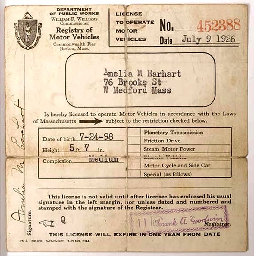
Driver’s licenses are commonly used as sources of foren-
The source routinely employed for Amelia Earhart’s height sic statures. Figure 4 shows Earhart’s Massachusetts driv-
has been her pilot’s license, where 5'8" is recorded. This is er’s license for 1927, where 5'7" is recorded. It is unlikely that90 Amelia Earhart and Nikumaroro Bones
the height on her driver’s license was measured. It is a foren- comparing her height to anthropometric data collected
sic stature that is as valid as the one on her pilot’s license. on Pembroke College Women in 1927 by A. M. Tousley and
This makes the point that height is not a fixed attribute that on University of Tennessee women measured in 1930 by
is measured or reported consistently. It was therefore neces- I. G. Carter, both series reported by Carter (1932). If Amelia
sary to seek a measured height which can be obtained pho- Earhart was 67 inches (170 cm) tall, she was taller than 85%
tographically by scaling her to known dimensions of an of Pembroke College women and 92% of University of Ten-
aircraft. Glickman (2016a) estimates her height at 67.125 nessee women. If she was 68 inches (172.7 cm) tall, she was
inches, almost an inch less than the height reported on her taller than 88% of Pembroke College women and 97% of
pilot’s license but in agreement with her driver’s license. University of Tennessee women. Males of her birth cohort
Glickman’s height has the advantage that it was measured, were 169.1 cm (Floud et al. 2011), so Earhart was slightly
the methods described, and it is subject to verification. While taller than the average male of her time.
the difference between the forensic heights and measured It turns out, too, that American “high society” women
height is relatively inconsequential, I will use the measured of the 19th century were substantially taller than average
height of 67 inches for the remainder of the paper. and seemed to be immune to the stature decline affecting
Whether she was 5'8" or 5'7", Earhart was a tall woman the general population (Sunder 2011). Sunder estimates the
for the time in which she lived. This can be illustrated by average height of high society women, which probably includes
FIG. 4—Amelia Earhart’s 1927 Massachusetts driver’s license showing her height as 5'7", one inch shorter than that
given on her pilot’s license.Jantz 91
Earhart, at the end of the 19th century at 64.9 inches (164.8 cm), significant but also too weak to discriminate robust from
more or less equal to what it is today. gracile skeletons using BMI.
The problem of course is that neither Cross and Wright
Relationship between BMI and Skeletal Robusticity (2015) nor anyone else has any idea how Hoodless made the
judgment that the skeleton was that of a stocky person. But
Cross and Wright (2015) argue that Amelia Earhart is what is clear is that the inference from BMI provides no basis
excluded because her physique was extremely linear and to exclude the bones as belonging to Amelia Earhart, Hood-
gracile, and therefore inconsistent with the skeletal remains less’s assessment notwithstanding.
which Hoodless assessed as belonging to a stocky individ-
ual. They argue, using height and weight (68 in. and 118 lb.) Amelia Earhart’s Body Build
from her pilot’s license, that Earhart’s body mass index
(BMI) is 17.9, placing her in the extreme lean range. From It is now possible to address the question of what Earhart’s
this they leap to infer a gracile skeleton that Hoodless would body build actually was, since it bears on what Hoodless may
not have mistaken for that of a stocky male. have seen before him. Cross and Wright (2015) characterize
There are two problems with this inference: (1) there is Earhart as tall, slender, and gracile, citing numerous photos
no necessary relationship between BMI and skeletal robus- of her to support this assessment. However, the few photos
ticity, and (2) available evidence does not support the infer- showing Earhart’s bare arms or legs (Figure 5) show a woman
ence that Earhart’s skeletal structure was gracile. I shall with a healthy amount of body fat. The photos in Figure 5
examine both of these in turn. are inconsistent with a weight of 118 pounds and a BMI of
The purpose of computing a BMI is to assess body fat, 17.9, which according to contemporary standards is in the
albeit an imperfect indicator. Since it is a ratio (weight/ underweight or undernourished category. If her height is
height2), all components of weight, including muscle and actually 5'7", that brings her BMI to 18.5, just to the lower
bone, in addition to fat, contribute to the value. Body pro- border of healthy weight. But even that is inconsistent with
portions also play a role (Norgan 1994). On average, how- the photos in Figure 5.
ever, higher BMIs correspond to more body fat. But what It is evident from Figure 5 that Earhart’s calves and
does that say about skeletal robusticity? There are several ankles cannot be described as slender. In the 1933 photo she
lines of evidence suggesting that the relationship is not is standing next to a woman somewhat taller, but with rather
close. more slender ankles. One of Earhart’s biographers, Susan
The size of articular surfaces is one measure of bone Butler (1997), recounts that because of her thick ankles, her
robusticity. In the FDB data, using forensic height and weight legs could be described as “piano legs.” Thick ankles are not
to calculate BMI, the humerus and femur head diameters, normally due to an undesirable distribution of fat; the sub-
femur epicondylar and tibia proximal breadths do not have cutaneous fat layer is normally thin, the ankle configuration
significant correlations with BMI. Normalizing them by bone owing to underlying bone and muscle (Weniger et al. 2004).
lengths increases the correlations slightly but they still do not Ankle circumference is often used as a measure of frame size
reach statistical significance. Ding et al. (2005) measured (Callaway et al. 1991). Calf and ankle circumference are
proximal tibia articular surface area from MRI scans and strongly correlated with weight (Cheverud et al. 1990a), the
compared it to BMI. The correlations were 0.25 and 0.16 for former reflecting mainly muscle and fat, the latter mainly
medial and lateral tibia articular surface areas, respectively. bone.
These correlations are statistically significant but so weak
they lack predictive power. Joint surface size is likely a good Empirical Estimation of Weight
indicator of lean body mass but has little to do with BMI.
Femur head size has a moderately high correlation with Weight can be estimated within reasonably tight limits if
weight and has been used to estimate weight in archeological appropriate information is available. Circumferences typi-
samples (Auerbach & Ruff 2004), which would not normally cally have the highest correlation with weight. The exten-
have excessive fat. However, height is weakly correlated with sive U.S. military anthropometric surveys provide the simple
weight, so the ratio of weight to height2 diminishes the rela- bivariate correlations of 259 variables (Cheverud et al. 1990a).
tionship with skeletal robusticity. These correlations and the means and standard deviations
Another measure of robusticity is the size of the mid- (Gordon et al. 1989) allow construction of a covariance
shaft in relation to length, already discussed above concern- matrix from which regression equations can be calculated.
ing Hoodless’s sexing method. Femur midshaft robusticity Waist circumference at the level of the umbilicus was
has a moderate correlation with BMI in our forensic database, used to estimate weight. It is above the rim of the pelvis and
0.46 for females and 0.44 for males, which is statistically corresponds to the level at which the trousers were worn.92 Amelia Earhart and Nikumaroro Bones
FIG. 5—Photos of Amelia Earhart showing body fat/body mass of arms and legs inconsistent with a weight
of 118 pounds. Photos courtesy of Remember Amelia, the Larry C. Inman Historical Collection on Amelia
Earhart.
Waist circumference obtained from Earhart’s trousers is Waist circumference alone estimates Earhart’s weight
27.375 inches (69.53 cm). The average for U.S. military women at slightly more than the weight given on her pilot’s license,
is 79.2 cm, about 10 cm larger than Amelia Earhart’s mea- but with a large error. Including height raises the estimate
surement. This supports what is evident from the photo- 10 pounds, to 129.7, and reduces the error more than a kilo-
graphic record, that she had a narrow body. Table 4 shows gram. The 90% confidence interval (114.8–144.3) includes
estimates of Earhart’s weight using waist circumference and the weight on her pilot’s license, but it is equally likely that
a height of 67 inches. she weighed somewhat more than 130 pounds.Jantz 93
TABLE 4—Regression estimates of Amelia Earhart’s weight using waist
circumference alone and waist circumference combined with height.
X Variables Estimated Weight RMS Error (kg) R2
Waist C.* 54.6 kg (119.9 lb.) 5.38 0.585
Ht, WC** 58.9 kg (129.7 lb.) 4.18 0.750
* Weight = 0.7724*wc + 0.8436.
** Weight = 0.5402*ht + 0.7022*wc − 81.8166.
Using a height of 67 inches and a weight of 130 pounds
yields a BMI of 20.4, a normal value very much in keeping
with the photographic evidence in Figure 5. The calf and
ankle morphology may also suggest that her limb bones were
not as gracile as supposed by Cross and Wright (2015) based
on their assessment of her BMI. Unfortunately, we have only
photographic and anecdotal evidence of Earhart’s ankle and
calf size, but Butler’s (1997) characterization suggests that
they exceeded those of most women of her height and weight.
Estimation of Humerus and Radius Length
Among the many photos of Amelia Earhart is one showing her
standing with right arm fully extended holding a can of Mobile
Lubricant (Figure 6). An exemplar of the can was obtained by
Jeff Glickman of Photek. A known dimension of the oil can
provides a scale allowing the pixel coordinates of points on
Earhart’s arm to be converted to linear distances (Glickman
2017). The major difficulty is identifying osteological points
underlying the soft tissue. Figure 6 shows the locations for
proximal and distal humerus and radius estimated to corre-
spond to measuring points on dry bones. It is not possible to
locate these points exactly, but they should provide reason-
able approximations. The points shown in Figure 6 yield a
humerus length of 321.1 mm and a radius length of 243.7 mm,
compared to 325 and 245 for the corresponding Nikumaroro
bones. The brachial index obtained from these estimate is
75.9, which compares favorably to the 76 obtained by Glick-
man on a different photograph (Glickman 2016b)
Estimation of Tibia Length FIG. 6—Amelia Earhart with right arm extended and points marked
where humerus head, distal humerus, proximal radius and distal radius
Estimating Amelia Earhart’s tibia length is more problem- were located. Photo courtesy of Purdue Special Collections, Amelia
atic than the radius and humerus because we have not iden- Earhart Papers, George Putnam Collection.
tified a photo showing her lower leg allowing identification
of osteological points and a scalable object. Therefore, two
regression methods have been used: (1) estimating from stat- Substituting Glickman’s measured height of 67 inches
ure and (2) estimating from inseam length of Earhart’s trou- (170.18 cm) into the equation yields a point estimate of
sers. Estimating from stature is straightforward and was 372.4 mm.
accomplished by regressing tibia length on stature using Estimating from inseam length is less straightforward
females from our database. The equation is: and involves using regression equations from U.S. military
anthropometric data. Unfortunately, a direct measurement of
Tibia length = 2.1601 (height) + 4.8335 ± 12.50 tibia length is not included in the military data. The two94 Amelia Earhart and Nikumaroro Bones
dimensions most closely approximating my needs are crotch Fordisc for 19th-century males, WW2 males, and 20th-cen-
height and lateral femur epicondyle height. The procedure is tury males. Noonan’s height falls outside the 90% confidence
as follows: intervals for all nine estimates, and outside the 95% for five
of the nine estimates. It is clear that the Nikumaroro bones
1. Adjust inseam length to crotch height by adding are unlikely to have belonged to Noonan.
ankle height. This assumes that Earhart’s trouser legs Eleven men were killed at Nikumaroro in the 1929 wreck
were level with the sphyrion landmark, the tip of the of the Norwich City on the island’s western reef, something
fibula. Earhart’s inseam measurement is 28.625 inches, over four miles from where the bones were found in 1940.5
or 727 mm. The ankle height adjustment, obtained from This number included two British and five Yemeni that were
Cheverud et al. (1990b), is 63 mm, making Earhart’s unaccounted for, but we have no documentation on them and
crotch height = 727 + 63 = 790 mm. there is no evidence that any survived to die as a castaway.
2. Estimate Earhart’s lateral femur condyle height using The woman’s shoe and the American sextant box are not arti-
regression equation in Cheverud et al. (1990b:780). The facts likely to have been associated with a survivor of the
equation is: Norwich City wreck. If an Islander somehow ended up as a
Lateral femur epicondyle height = 0.526 (crotch height) + castaway, there is likewise no evidence of this.
55.195 ± 8.53 If the skeleton were available, it would presumably be a
Substituting 790 mm yields a point estimate of 470.7 mm. relatively straightforward task to make a positive identifica-
3. Adjust lateral femur condyle height to tibia length by tion, or a definitive exclusion. Unfortunately, all we have are
subtracting ankle height (63 mm, as above) and femur the meager data in Hoodless’s report and a premortem record
distal condyle height, 36 mm (Simmons et al. 1990). gleaned from photographs and clothing. From the informa-
The point estimate is 470.7 − 63 − 36 = 371.7. tion available, we can at least provide an assessment of how
well the bones fit what we can reconstruct of Amelia Earhart.
There are admittedly several adjustments involved in Because the reconstructions are now quantitative, probabil-
this process, but they are all reasonable. Most of the varia- ities can also be estimated.
tion in lateral condyle height involves tibia length, so minor Estimates of humerus, radius, and tibia lengths obtained
variation in adjustments will not have major influence on the from Amelia Earhart allow one to proceed as one normally
estimate. Crotch height has a much higher correlation with would in a forensic situation. The Nikumaroro remains can
femur lateral condyle height, and hence with tibia length, now be compared to Amelia Earhart to address the question of
than height. However, the estimates from height and lateral whether she can be excluded or included. It is already apparent
femur condyle height are very similar, 372.4 versus 371.7, so that Earhart’s vector of measurements, [321.1,243.7,372] is sim-
I will take 372 mm as the estimate of Earhart’s tibia length. ilar to that of the Nikumaroro bones [325,245,372]. These vec-
tors contain both size and shape information, so a comparison
Do the Nikumaroro Bones Fit Amelia Earhart? should capture both of those elements. This was accomplished
by computing Mahalanobis distance (D) of 2,776 individu-
When confronted with human remains of unknown origin, als in our postcranial database from the Nikumaroro bones.
the procedure followed in ordinary forensic practice is to Amelia Earhart’s data were included to yield N = 2,777.
develop a biological profile, and from among missing per- Figure 7 displays a histogram of the distances, by sex,
sons, select those that fit the profile. At that point one attempts of 2,777 individuals from the Nikumaroro bones. The verti-
to make a positive identification by using features seen on cal line shows Earhart’s position in the two distributions. She
the bones that can also be seen in premortem records of the is clearly in the left tail of both distributions, but more so for
possible victims. The premortem records may consist of den- females. Her z-score in the female distribution is − 2.38 ( p =
tal or frontal sinus images, or increasingly, DNA taken from 0.017) and in the male distribution − 1.87 ( p = 0.061). She has
remains and comparing to the victim or relatives of the vic- a low probability of coming from the male distribution and
tim. A positive identification is made when premortem fea- a much lower one for the female distribution. Earhart is in
tures match the victim and have a low probability of matching the first bin of the histogram for females, along with only two
anyone else. other females (0.526%). There are 16 males in the first bin
In the case of the Nikumaroro bones, the only docu- (0.725%)
mented person to whom they may belong is Amelia Earhart. One might argue that if the Nikumaroro bones are actu-
Her navigator, Fred Noonan, can be reliably excluded on the ally those of Amelia Earhart, the distance should be zero,
basis of height. His height was 6'1/4", documented from his but that expectation is unrealistic for at least two reasons:
1918 Seaman’s Certificate of American Citizenship. I made
nine stature estimates of the Nikumaroro bones, three each 5. See https://tighar.org/Projects/Earhart/Archives/Research/Research
for the humerus, radius, and tibia, using male equations in Papers/WreckNorwichCity.html.Jantz 95
combination of bone lengths has considerable power to
individualize.
Earhart’s rank is 19, meaning that 2,758 (99.28%) indi-
viduals have a greater distance from the Nikumaroro bones
than Earhart, but only 18 (0.65%) have a smaller distance.
The rank is subject to sampling variation, so I conducted
1,000 bootstraps of the 2,776 distances, omitting Earhart,
then replacing her to determine her rank. Her rank ranged
from 9 to 34, the 95% confidence intervals ranging from 12
to 29. If we take the maximum rank resulting from 1,000
bootstraps, 98.77% of the distances are greater and only
1.19% are smaller. If these numbers are converted to likeli-
hood ratios as described by Gardner and Greiner (2006), one
obtains 154 using her rank as 19, or 84 using the maximum
bootstrap rank of 34. The likelihood ratios mean that the
Nikumaroro bones are at least 84 times more likely to belong
to Amelia Earhart than to a random individual who ended up
on the island.
The Gardener and Greiner method requires intervaliz-
ing a continuous distribution. The above procedure dichoto-
mized the distribution, breaking it at Earhart’s rank, and at
FIG. 7—Histograms of 2,777 Mahalanobis distances (D) from the the maximum bootstrap rank. It might be argued that this
Nikumaroro bones, by sex. The line shows Earhart’s position in the weights the result in favor of similarity of Earhart to the
distribution. Nikumaroro bones. Even if one breaks the distribution into
deciles, the likelihood ratio is still 10. Regardless of how one
(1) it would require that my estimates of bone lengths were chooses to break the distribution, the fact remains that Ear-
made without error, which is highly unlikely, and (2) it hart is more similar to the Nikumaroro bones than all but a
would require that Hoodless measured the Nikumaroro small fraction of random individuals.
bones without error, which is also unlikely. The above analysis considers only the comparison of
It should be mentioned that a sample of Micronesian or Earhart to the Nikumaroro bones in relation to every other
Polynesian bone measurements was unavailable to test distance from Nikumaroro in our database. A more robust
against the Nikumaroro bones. I consider it highly unlikely distribution of distances can be obtained by randomly sam-
that inclusion of such a sample would have changed anything. pling individuals from the database and comparing them to
As Figure 3 shows, the Nikumaroro bones are more similar the sample as described above. Each randomly sampled indi-
to Euro-Americans than they are Micronesians or Polyne- vidual serves as an unknown in the same manner as the
sians, which suggests they would produce even fewer near- Nikumaroro bones in the previous analysis. I randomly sam-
est neighbors. pled 500 individuals from the database, omitting each ran-
Another approach to the question is to examine Earhart’s domly sampled individual in turn from the comparison
rank in the distributions. For clarity, I should point out that because it would obviously have zero distance from itself.
if any individual in our sample had a vector of measurements Sex was ignored for this exercise. From the 500 randomly
identical to the Nikumaroro bones, the distance would be sampled individuals, 17 had zero distance from another indi-
zero and have a rank of one, that is, most similar to the Niku- vidual, that is, had an identical vector of measurements. One
maroro bones. But not one from our 2,776 individuals had a had an identical vector with two individuals, giving a total
vector identical to Nikumaroro’s. The lowest Mahalanobis of 19 identical vectors from the 500 random samples, or 3.8%.
distance is 0.12599, resulting from a vector of [322,243,369]. This illustrates that identical vectors are a comparatively rare
That vector is noteworthy because its elements are uniformly event. Summary statistics of the means, standard deviations,
shorter than Nikumaroro, 3 mm for humerus and tibia and minima and maxima obtained from the 500 random samples
2 mm for radius. Hence the most similar individual is almost are shown in Table 5. The summary statistics of the Niku-
identical in shape but differs slightly in size. The largest dis- maroro bones are included for comparison.
tance is 4.57, from a vector of [361,252,430]. It is larger The data in Table 5 reveal that the entire 500 randomly
than Nikumaroro in all dimensions, but shape still domi- sampled individuals have limited similarity to any other
nates because the differences range from only 9 mm (radius) bones in the sample. The mean of the 500 means (2.2268) is
to 58 mm (tibia). These examples suggest that the particular somewhat higher than that for the Nikumaroro comparison,96 Amelia Earhart and Nikumaroro Bones
TABLE 5—Descriptive statistics of Mahalanobis distances (D) for 500 they still exist) those of Amelia Earhart. If the bones do not
randomly sampled individuals from 2,775 individuals in the database. belong to Amelia Earhart, then they are from someone very
Descriptive Statistics of 500 Random Samples for
similar to her. And, as we have seen, a random individual has
a very low probability of possessing that degree of similarity.
Means SDs Minima Maxima
Ideally in forensic practice a posterior probability that
Mean 2.2268 0.82167 0.1681 5.4836 remains belong to a victim can be obtained. Likelihood ratios
SD 0.4545 0.0727 0.1046 0.6665
Min 1.5777 0.6590 0 4.2496 can be converted to posterior odds by multiplying by the prior
Max 4.4622 0.9684 0.8277 8.2367 odds. For example, if we think the prior odds of Amelia Ear-
Nikumaroro 1.6969 0.7338 0.1260 4.5700
hart having been on Nikumaroro Island are 10:1, then the
likelihood ratios given above become 840–1,540, and the
and the average minimum (0.1681) is also higher than the posterior probability is 0.999 in both cases. The prior odds
Nikumaroro comparison. But the Nikumaroro statistics are or prior probability pertain to information available before
within the range of the 500 randomly sampled individuals. skeletal evidence is considered. It is often impossible to
That the Nikumaroro comparison has somewhat lower dis- assign specific numbers to the prior probability, because it
tances only means that the Nikumaroro bones are closer to depends on how the non-osteological evidence is evaluated,
the average than many of the randomly sampled individuals. and different people will usually evaluate it differently. In
jury trials, experts are often advised to testify only to the
likelihood ratio developed from the biological evidence. The
Discussion jury then supplies its own prior odds based on the entire con-
text (e.g., Steadman et al. 2006).
Let us suppose, for the sake of argument, that the Nikuma- In the present instance, readers can supply their own
roro bones are the remains of Amelia Earhart. In light of the interpretation of the prior evidence, summarized by King
above, we can now reconsider what Hoodless might have (2012). Given the multiple lines of non-osteological evidence,
seen before him and how he might have assessed what he it seems difficult to conclude that Earhart had zero probabil-
saw. The skeleton before him would have had bone lengths ity of being on Nikumaroro Island. From a forensic perspec-
clearly in the male range. From what we see of Earhart’s tive the most parsimonious scenario is that the bones are
lower leg morphology, it is quite possible, even likely, that those of Amelia Earhart. She was known to have been in the
the tibia was relatively robust. As a tall and narrow-bodied area of Nikumaroro Island, she went missing, and human
female, the “set” of the femora could well have appeared male remains were discovered which are entirely consistent with
to Hoodless. It is apparent from the many photos of Earhart, her and inconsistent with most other people. Furthermore, it
and from her waist circumference, that her hips were narrow is impossible to test any other hypothesis, because except for
for a female. This, in combination with her height, does not the victims of the Norwich City wreck, about whom we have
require a femur angle one might expect of a female. It may no data, no other specific missing persons have been reported.
also suggest an ambiguous half subpubic angle that could It is not enough merely to say that the remains are most likely
easily have been called male by an inexperienced eye, or even those of a stocky male without specifying who this stocky
an experienced one, particularly if taphonomic processes had male might have been. This presents us with an untestable
modified the morphology. hypothesis, not to mention uncritically setting aside the prior
If Hoodless’s analysis, particularly his sex estimate, can be information of Earhart’s presence. The fact remains that if
set aside, it becomes possible to focus attention on the central the bones are those of a stocky male, he would have had bone
question of whether the Nikumaroro bones may have been lengths very similar to Amelia Earhart’s, which is a low-prob-
the remains of Amelia Earhart. There is no credible evidence ability event. Until definitive evidence is presented that the
that would support excluding them. On the contrary, there remains are not those of Amelia Earhart, the most convinc-
are good reasons for including them. The bones are consis- ing argument is that they are hers.
tent with Earhart in all respects we know or can reasonably
infer. Her height is entirely consistent with the bones. The
skull measurements are at least suggestive of female. But Acknowledgments
most convincing is the similarity of the bone lengths to the
reconstructed lengths of Earhart’s bones. Likelihood ratios Many colleagues, friends, and family members have contrib-
of 84–154 would not qualify as a positive identification by uted to this paper in various ways. Ric Gillespie and
the criteria of modern forensic practice, where likelihood TIGHAR’s resources enabled me to get information from
ratios are often millions or more. They do qualify as what is Amelia Earhart’s clothing and from photographs allowing
often called the preponderance of the evidence, that is, it is quantification of several aspects of her body size and limb
more likely than not the Nikumaroro bones were (or are, if lengths and proportions. Ric also answered many questionsYou can also read