Asset Bubbles and Bailout - CARF Working Paper
←
→
Page content transcription
If your browser does not render page correctly, please read the page content below
CARF Working Paper

                                             CARF-F-268

                            Asset Bubbles and Bailout
                                         Tomohiro Hirano
                                      The University of Tokyo
                                           Masaru Inaba
                                         Kansai University
                                        Noriyuki Yanagawa
                                      The University of Tokyo

                                     First version: January 2012
                                   Current version: December 2012

    CARF is presently supported by Bank of Tokyo-Mitsubishi UFJ, Ltd., Dai-ichi Mutual Life
    Insurance Company, Meiji Yasuda Life Insurance Company, Nomura Holdings, Inc. and
    Sumitomo Mitsui Banking Corporation (in alphabetical order). This financial support enables
    us to issue CARF Working Papers.

                 CARF Working Papers can be downloaded without charge from:
                    http://www.carf.e.u-tokyo.ac.jp/workingpaper/index.cgi

Working Papers are a series of manuscripts in their draft form. They are not intended for
circulation or distribution except as indicated by the author. For that reason Working Papers may
not be reproduced or distributed without the written consent of the author.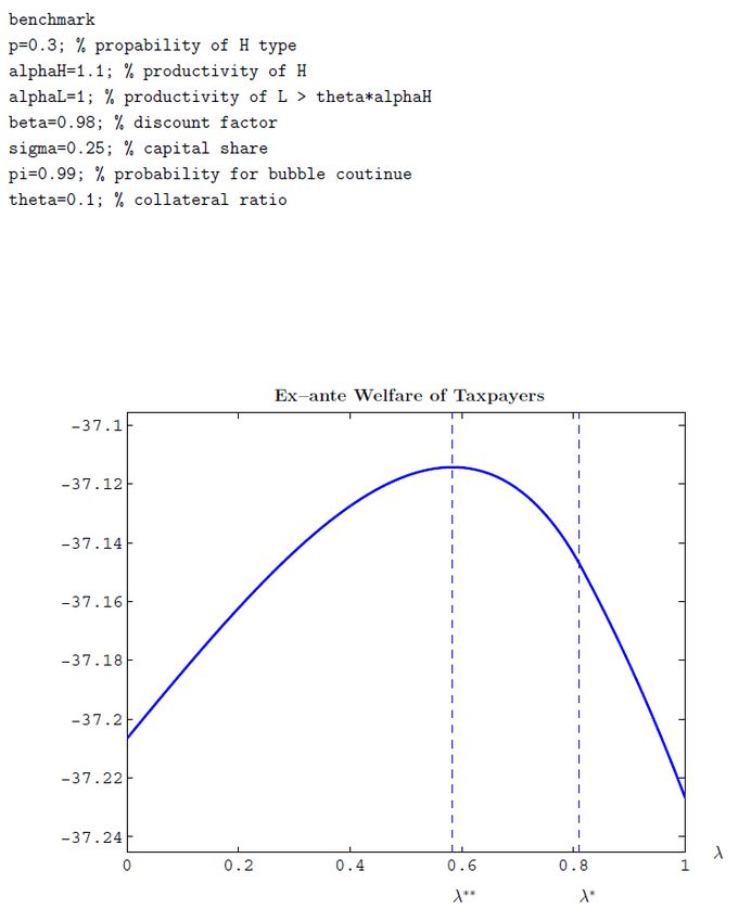
Asset Bubbles and Bailout
   Tomohiro Hirano, Masaru Inaba, and Noriyuki Yanagawa

                         First Version, April 2011
                       This Version, September 2012

                                       Abstract
          This paper theoretically investigates the relationship between gov-
      ernment bailout and asset bubbles. We show that even riskier bub-
      bles are more likely to occur, the more bailout is anticipated. We also
      analyze to what extent is ex-post bailout desirable from ex-ante e¢ -
      ciency in production. We show that expansion of the bailout initially
      enhances ex-ante e¢ ciency in production and then decreases it. Fur-
      thermore, we analyze how the anticipated bailout a¤ects boom-bust
      cycles. We show that anticipated bailout ends up with increasing
      boom-bust cycles and requiring large amount of public funds in the
      bubbles’ collapsing. Finally, we derive an optimal bailout policy for
      tax payers. We show that partial bailout is optimal, in the sense that
      no-bailout is not optimal and rescuing all is not optimal neither. In
      the case of riskier bubbles, government has to give up some e¢ ciency
      in production, so that even unproductive entrepreneurs produce and
      boom-bust cycles become milder.

    This is a revised version of our previous working paper, Hirano, Tomohiro and Noriyuki
Yanagawa. (2012 January) "Asset Bubbles and Bailout". To revise our paper, we have
bene…ted greatly from discussions with Harald Uhlig. We also thank Nobuhiro Kiyotaki,
Kosuke Aoki, Je¤rey Campbell, Koichi Hamada, Fumio Hayashi, Hugo Hopenhayn, Tat-
suro Iwaisako, Takashi Kamihigashi, Kiminori Matsuyama, Albert Martin, Jianjun Miao,
Penfei Wang, Kalin Nikolov, Fabrizio Perri, Masaya Sakuragawa, and seminar participants
at 2012 Econometric Society North American Summer Meeting, European Economic As-
sociation Meeting, 2012 Midwest Macroeconomics Meeting, 2012 saet conference, and 2012
Royal Economic Society.

                                            1
1       Introduction
Many countries have experienced bubble-like dynamics. Associated with the
bursting part of asset price bubbles are signi…cant contractions in real eco-
nomic activity. Notable examples include the recent U.S. experiences after
the …nancial crisis of 2007/2008 as well as Japan’s experiences in the 1990s.
To mitigate severe contractions, government tends to take various types of
bailouts such as recapitalization through buying equity or through the pur-
chase of troubled assets at in‡ated prices. Although these policies may miti-
gate the contractions ex-post, what happens if these policies are anticipated
ex-ante? In this paper, we ask the following questions.

        How does anticipated bailout a¤ect the emergence of asset bubbles?

        To what extent is ex-post bailout desirable from ex-ante perspective?

        How does anticipated bailout a¤ect boom-bust cycles?

        Finally, we derive an optimal bailout policy for tax payers.

    For this purpose, we develop a macroeconomic model with stochastic
bubbles.1 The recent developments on rational bubbles have provided a the-
oretical framework to analyze asset price bubbles (Caballero and Krishna-
murthy, 2006; Farhi and Tirole, 2009; Kocherlalota, 2009; Hirano and Yana-
gawa, 2010a, 2010b; Martin and Ventura, 2010a, 2010b; Aoki and Nikolov,
2011; Miao and Wang, 2011). We extend a rational bubble model to include
bailout. In the present paper, since bubble assets are risky in the sense that
bubbles may collapse, risk-averse entrepreneurs want to hedge themselves
by investing in safe assets. As we show, the entrepreneurs’ portfolio deci-
sion depends upon not only the bursting probability of bubbles, but also the
expectations about the government policy.
    What is new in our framework is that through the change in risk-taking
behaviors of the entrepreneurs, the anticipated bailout a¤ects the emergence
of asset price bubbles, ex-ante e¢ ciency in production, and boom-bust cy-
cles. We show that even riskier bubbles are more likely to occur, the more
bailout is anticipated. We also show that expansion of the bailout initially
enhances ex-ante e¢ ciency in production and then decreases it. Furthermore,
    1
   Weil (1987) is the …rst study that analyzes stochastic bubbles in a general equilibrium
model.

                                            2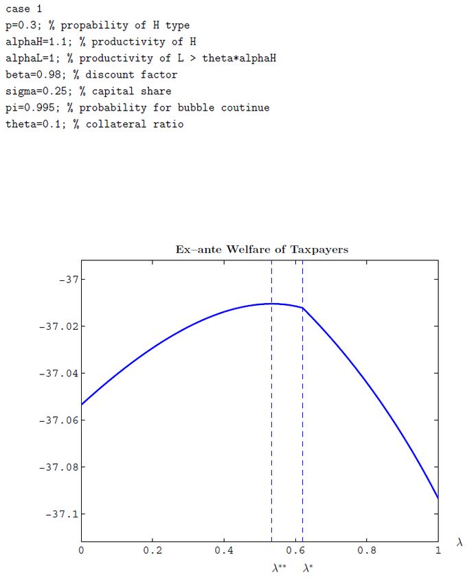
we show that anticipated bailout ends up with increasing boom-bust cycles
and requiring large amount of public funds in the bubbles’collapsing.
    Finally, we derive an optimal bailout policy for tax payers. We show that
partial bailout is optimal, in the sense that no-bailout is not optimal and
rescuing all is not optimal neither. This result has implications for boom-
bust cycles. In the case of riskier bubbles, government has to give up some
e¢ ciency in production, so that even unproductive entrepreneurs produce
and boom-bust cycles become milder.
    Our paper is related to theoretical literature that examines government
bailouts and risk-taking. For example, Chari and Kehoe (2010), Diamond
and Rajan (2011), and Farhi and Tirole (2011) stress moral hazard conse-
quences of bailouts and other credit market interventions in a three-period
model. Our paper is mainly di¤erent from these papers in the point that
we analyze bailout within a full blown dynamic macroeconomic model. In
this respect, our paper is closely related to Gertler et al. (2011). Gertler et
al. show (2011) that anticipated monetary poicy induces banks to adopt a
riskier balance sheet ex-ante, which will in turn require a larger scale credit
market intervention during a crisis. They also analyze regulations that mit-
igates moral hazard and improves welfare. On the other hand, we derive an
optimal bailout policy for tax papers in a rational bubbles model.

2     The Model
2.1    Framework
Consider a discrete-time economy with one homogeneous good and a contin-
uum of entrepreneurs and workers. A typical entrepreneur and a representa-
tive worker have the following expected discounted utility,
                                "1             #
                                 X
                                      t
                             E0         log cit ;                      (1)
                                  t=0

where i is the index for each entrepreneur, and cit is the consumption of
him/her at date t. 2 (0; 1) is the subjective discount factor, and E0 [a] is
the expected value of a conditional on information at date 0.
   Let us start with the entrepreneurs. At each date, each entrepreneur
meets high productive investment projects (hereinafter H-projects) with prob-

                                        3
ability p, and low productive ones (L-projects) with probability 1 p.2 The
investment projects produce capital. The investment technologies are as fol-
lows:
i
kt+1 = it zti ; (2)
where zti ( 0) is the investment level at date t; and kt+1
i
is the capital at
i
date t + 1 produced by the investment. t is the marginal productivity
of investment at date t. it = H if the entrepreneur has H-projects, and
i L
t = if he/she has L-projects. We assume H > L . For simplicity,
we assume that capital fully depreciates in one period.3 The probability
p is exogenous, and independent across entrepreneurs and over time. At
the beginning of each date t, the entrepreneur knows his/her own type at
date t, whether he/she has H-projects or L-projects. Assuming that the
initial population measure of each type of the entrepreneur is p and 1 p
at date 0, the population measure of each type after date 1 is p and 1
p, respectively. Throughout this paper, we call the entrepreneurs with H-
projects "H-entrepreneurs" and the ones with L-projects "L-entrepreneurs".
We assume that because of frictions in a …nancial market, the entre-
preneur can pledge at most a fraction of the future return from his/her
investment to creditors.4 In such a situation, in order for debt contracts to
be credible, debt repayment cannot exceed the pledgeable value. That is, the
borrowing constraint becomes:
rt bit qt+1 it zti ; (3)
where qt+1 is the relative price of capital to consumption goods at date t + 1.5
rt and bit are the gross interest rate and the amount of borrowing at date t,
respectively. The parameter 2 (0; 1], which is assumed to be exogenous, can
be naturally taken to be the degree of imperfection of the …nancial market.
In this economy, there are bubble assets denoted by x. Aggregate supply
of the assets is assumed to be constant over time X: As in Tirole (1985),
2
A similar setting is used in Woodford (1990), Kiyotaki (1998), Kiyotaki and Moore
(2008), Kocherlakota (2009).
3
As in Kocherlakota (2009), we can consider a situation where some fraction of capital
depreciate, and consumption goods can be converted one-for-one into capital at each date,
and vice-versa. In this setting, we can also obtain the same results as in the present papar.
4
See Hart and Moore (1994) and Tirole (2006) for the foundations of this setting.
5
On an equilibrium path we consider, qt+1 is not a¤ected by whether bubbles collapse
or not. Hence, there is no uncertainty with regard to qt+1 :
4we de…ne bubble assets as the assets that produce no real return, i.e., the
fundamental value of the assets is zero. Following Weil (1987), we consider
stochastic bubbles, in the sense that they may collapse. In each period t;
bubble prices become zero (bubbles burst) with probability 1 conditional
on survive at date t 1: Once they burst, they never arise again. This implies
that bubbles persist with probability (< 1) and their prices are positive until
they switch to being equal to zero forever. Let Pt be the per unit price of
bubble assets at date t on survive in terms of consumption goods.
The entrepreneur’s ‡ow of funds constraint is given by
cit + zti + Pt xit = qt i i
t 1 zt 1 rt 1 bit 1 + bit + Pt xit 1 + mit : (4)
where xit be the level of bubble assets purchased by a type i entrepreneur at
date t. The left hand side of (4) is expenditure on consumption, investment,
and the purchase of bubble assets. The right hand side is the available
funds at date t, which is the return from investment in the previous period
minus debts repayment, plus new borrowing, the return from selling bubble
assets, and bailout money, mit . We assume that the bailout is proportional
of holdings of the bubble assets.
mit = dt xit 1 : (5)
When bubbles collapse, a fraction 2 [0; 1] of the entrepreneurs who hold
bubble assets is rescued. = 0 means that no-entrepreneur is rescued.
= 1 means that all are rescued. Thus a rise in means expansion of the
bailout. From ex-ante perspective, each entrepreneur anticipates the govern-
ment bailout with probability : When the entrepreneur is rescued, he/she
gets dt units of consumption goods per unit of bubble assets. Otherwise,
he/she gets nothing. We de…ne the net worth of the entrepreneur at date t
as
eit qt it 1 zti 1 rt 1 bit 1 + Pt xit 1 + mit :
We also impose the short sale constraint on bubble assets:6
xit 0: (6)
Let us now turn to the workers. There are workers with a unit measure.
6
Kocherlakota (1992) shows that the short sale constraint plays an important role for
the emergence of asset bubbles in an endowment economy with in…nitely lived agents.
5Each worker is endowed with one unit of labor endowment in each period,
which is supplied inelastically in labor markets, and earns wage rate, wt .
The ‡ow of funds constraint, the borrowing constraint, and the short sale
constraint for them are given by
cut + Pt (xut xut 1 ) = wt rt 1 but 1 + but Tt ; (7)
rt but 0; (8)
xut 0; (9)
where u represents the workers. Tt is a lump sum tax.7 When bubbles
collapse, the government levies the lump sum tax on workers, and transfers
those funds to entrepreneurs. This means that workers pay direct costs of
the bubbles’ collapsing. Thus we call workers "tax payers". Tt > 0 only
when bubbles collapse. Tt = 0 if they survive: As in Farhi and Tirole (2012),
the aim of this bailout policy is to boost the net worth of entrepreneurs.
Equation (8) says that workers cannot borrow, since they do not have any
collateralizable assets such as returns from investment projects.
There are competitive …rms which produce …nal consumption goods using
capital and labor.8 The production function of each …rm is
yt = kt nt1 : (10)
Factors of production are paid their marginal product:
1
qt = K t and wt = (1 )Kt ; (11)
where K is the aggregate capital stock.
7
In order to focus on a transfer policy from workers to entrepreneurs as in Farhi and
Tirole (2012), we do not consider a tax on entrepreneurs. Even if we consider the capital
income tax, we can obtain the same results as in the main text, although the borrowing
constraint for entrepreneurs and the investment function would be complicated as analyzed
in Aoki et al. (2009).
8
We assume that each …rm is operated by the workers. Since the …nal goods market
is competitive, the net pro…t from operating the …rm is zero, so that the ‡ow of funds
constraint of the workers is unchanged as equation (6) in equilibirum.
62.2 Equilibrium
Let us denote theP aggregate consumption
P of H-and L-entrepreneurs and work-
ers at date t as i2Ht ct Ct , i2Lt ct CtL , Ctu ; where H
i H i
Pt and L t mean
i
a
Pfamilyi of H-and PL-entrepreneurs at date t. Similarly, let
P P i2Ht zit ZtH ;
L i H i L u
Pi2Lt zt i
Zt ;
u
i2Ht bt Bt ; i2Lt bt Bt ; Bt ; i2Ht [Lt kt Kt ;
( i2Ht [Lt xt + Xt ) Xt be the aggregate investment, the aggregate borrow-
ing, the aggregate capital stock, and the aggregate demand for bubble assets.
Then the market clearing condition for goods, credit, labor, and bubble assets
are
CtH + CtL + Ctu + ZtH + ZtL = Yt ; (12)
BtH + BtL + Btu = 0; (13)
Nt = 1; (14)
Xt = X: (15)
The competitive equilibrium is de…ned as a set of prices frt ; wt ; Pt g1 and
t=0
H L u H L u H L 1
quantities Ct ; Ct ; Ct ; Bt ; Bt ; Bt ; Zt ; Zt ; Gt ; Xt ; Kt+1 ; Yt t=0 , such that
(i) the market clearing conditions, (12)-(15), are satis…ed in each period,
and (ii) each entrepreneur chooses consumption, borrowing, investment, and
1
the amount of bubble assets, fcit ; bit ; zti ; xit gt=0 ; to maximize his/her expected
discounted utility (1) under the constraints (2)-(6), taking the bursting prob-
ability of bubbles and the bailout probability into consideration. (iii) each
worker chooses consumption, borrowing, and the amount of bubble assets,
fcut ; but ; xut g1
t=0 ; to maximize his/her expected discounted utility (1) under the
constraints (7)-(9), taking the bursting probability into consideration.
2.3 Optimal Behavior of Entrepreneurs and Workers
We now characterize the equilibrium behavior of entrepreneurs and workers.
We consider the case
qt+1 L rt < qt+1 H :
In equilibrium, interest rate must be at least as high as qt+1 L , since nobody
lends to the projects if rt < qt+1 L .
For workers, both the borrowing constraint and the short sale constraint
become binding in equilibrium. Thus, they consume all the wage income in
7each period. We later verify this in Appendix. That is,
cut = wt Tt :
Tt > 0 only when bubbles collapse.
For H-entrepreneurs at date t, both the borrowing constraint and the
short sale constraint simultaneously become binding. Since the utility func-
tion is log-linear, each entrepreneur consumes a fraction 1 of the net
i i 9
worth in each period, that is, ct = (1 )et . Then, by using (3), (4), and
(6), the investment function of H-entrepreneurs at date t can be written as
eit
zti = : (16)
qt+1 H
1
rt
This is a popular investment function under …nancial constraint problems, ex-
cept that the presence of bubble assets and government bailout a¤ect the net
worth.10 We see that the investment equals the leverage, 1= 1 ( qt+1 H =rt ) ,
times a fraction of the net worth. From this investment function, we un-
derstand that for the entrepreneurs who purchased bubble assets in the pre-
vious period, they are able to sell those assets at the time they encounter
H-projects. As a result, their net worth increases (compared to the bubbleless
case), which relaxes the borrowing constraint and boosts their investments.
That is, bubbles generate balance sheet e¤ects. Moreover, the expansion
level of the investment is more than the direct increase of the net worth
because of the leverage e¤ect. In our analysis, the entrepreneurs buy risky
bubble assets when they have L-projects, and sell those assets when they
have opportunities to invest in H-projects.
For L-entrepreneurs at date t, both the borrowing constraint and the
short sale constraint do not become binding. Instead, they decide optimal
portfolio choices. Since bubble assets deliver no return with probability 1 ,
risk-averse L-entrepreneurs may want to hedge themselves by investing in L-
projects as well as lending to other entrepreneurs. Since cit = (1 )eit ; the
budget constraint (4) becomes
zti + Pt xit bit = eit : (17)
9
See, for example, chapter 1.7 of Sargent (1988).
10
See, for example, Bernanke and Gertler (1989), Bernanke et al. (1999), Holmstrom
and Tirole (1998), Kiyotaki and Moore (1997), and Matsuyama (2007, 2008).
8Each L-entrepreneur allocates his/her savings, eit ; into zti ; Pt xit ; and bit : Since
investing in L-projects and lending are both safe assets, zti 0 if rt = qt+1 L ;
and zti = 0 if rt > qt+1 L : That is, the following conditions must be satis…ed:
L
(rt qt+1 )zti = 0; zti 0; and rt qt+1 L
0:
Each L-entrepreneur chooses optimal amounts of bit ; xit ; and zti ; so that the
expected marginal utility from investing in three assets is equalized. The
…rst order conditions with respect to bit and xit are
1 rt rt rt
(bit ) : = i; + (1 ) + (1 )(1 ) ; (18)
cit ct+1 i;(1
ct+1
) i;(1
ct+1
)(1 )
1 1 Pt+1 1 dt+1
(xit ) : = + (1 ) ; (19)
cit ci;t+1
Pt i;(1
ct+1
) Pt
where ci;t+1 = (1 )(qt+1 L zti rt bit + Pt+1 xit ) is the date t + 1 consumption
when bubbles survive. The …rst term of the right hand side in equation
(18) and (19) represents the expected marginal utility from lending a unit
i;(1 )
and from buying a unit of risky bubble assets in this case. ct+1 = (1
L i i i
)(qt+1 zt rt bt +mt+1 ) is the date t+1 consumption when bubbles collapse
and the government rescues the entrepreneur. The second term of equation
(18) and (19) represents the expected marginal utility from lending a unit
i;(1 )(1 )
and from buying a unit of risky bubble assets in this case. ct+1 =
(1 )(qt+1 L zti rt bit ) is the date t + 1 consumption when bubbles collapse
and the government does not rescue the entrepreneur. The third term of
equation (18) represents the expected marginal utility from lending a unit
in this case.11 Pt+1 =Pt is the rate of return of bubbles on survive. In this
analysis, we consider the bailout that fully recovers the net worth of rescued
entrepreneurs, i.e., dt+1 = Pt+1 :12
11
Since the entrepreneur consumes a fraction 1 of the current net worth in each
period, the optimal consumption level at date t + 1 is independent of the entrepreneur’s
type at date t + 1: It only depends on whether bubbles collapse and whether government
rescues the entrepreneur.
12
In this model, on the saddle path, the following condition is satis…ed.
Pt+1 K
= t+1 :
Pt Kt
Since Pt ; Kt ; and Kt+1 are predetermined variables at the beginning of date t + 1; the
9From (17), (18), and (19), we can derive the demand function for risky
bubble assets of a type i L-entrepreneur:
( ) PPt+1 rt
Pt xit = Pt+1
t
eit ; (20)
Pt
rt
where ( ) + (1 ) :
The remaining fraction of savings is split across zti and bit :
[1 ( )] PPt+1
zti bit = Pt+1
t
eit :
Pt
rt
From (20), we see that an entrepreneurs’s portfolio decision depends upon
its perceptions of risk, which in turn depends upon both the probability of
bursting of bubbles ( ) and expectations about the government bailout ( ).
We obtain the following Proposition.
Lemma 1 xit is an increasing function of :
Lemma 1 means that when rises, the type i L-entrepreneur is will-
ing to buy more bubble assets. That is, the anticipated bailout induces
L-entrepreneurs to take on more risk, even though the potential probability
of the bubble bursts remain unchanged ( is unchanged).
2.4 Aggregation
We are now in a position to consider the aggregate economy. The great merit
of the expressions for each entrepreneur’s investment and demand for bubble
assets, zti and xit ; is that they are linear in period-t net worth, eit . Hence
aggregation is easy: we do not need to keep track of the distributions.
From (16), we can derive the aggregate H-investments:
pAt
ZtH = H
; (21)
qt+1
1
rt
government can know the bubble prices whey they survive at date t + 1, Pt+1 :
10wherePAt iqt Kt + Pt X is the aggregate wealth of entrepreneurs at date t;
and i2Ht et = pAt is the aggregate wealth of H-entrepreneurs at date t. Re-
call that the probability of meeting H-projects is independently distributed.
From this investment function, we see that the aggregate investments of H-
entrepreneurs depend upon asset prices, Pt ; as well as cash ‡ows from the
investment projects in the previous period, qt Kt . In this respect, this invest-
ment function is similar to the one in Kiyotaki and Moore (1997). There is a
signi…cant di¤erence. In the Kiyotaki-Moore model, the investment function
depends upon land prices which re‡ect fundamentals (cash ‡ows from the
present to the future), while in our model, it depends upon bubble prices.
Aggregate L-investments depend upon the level of the interest rate.
8
pAt
>
> At Pt X if rt = qt+1 L ;
>
<
H
1
ZtL = L (22)
>
>
>
: 0 if rt > qt+1 L :
When rt = qt+1 L ; L-entrepreneurs may invest. In this case, aggregate L-
investments are determined by the goods market clearing condition (12).
They are equal to aggregate savings of the economy minus aggregate H-
investments minus aggregate value of bubbles. When rt > qt+1 L ; L-entrepreneurs
do not invest.
The aggregate counterpart to (20) is
( ) PPt+1
t
rt
Pt Xt = Pt+1
(1 p)At ; (23)
Pt
rt
P
where i2Lt eit = (1 p)At is the aggregate net worth of L-entrepreneurs at
date t: (23) is the aggregate demand function for bubble assets at date t:
2.5 Dynamics
Using (21) and (22), we can derive the evolution of aggregate capital stock:
8
>
>
< H pAtH + L At pAt
H Pt X if rt = qt+1 L ;
1 L 1 L
Kt+1 = (24)
>
>
: H
[ At Pt X] if rt > qt+1 L :
11The …rst term and the second term in the …rst line represent the capital stock
at date t + 1 produced by H-and L-entrepreneurs: When rt > qt+1 L ; only
H-entrepreneurs invest. From the goods market clearing condition, we know
ZtH = At Pt X: ( Pt X) in (24) captures a traditional crowd-out e¤ect
of bubbles (Tirole, 1985), i.e., L-entrepreneurs buy bubbles, which crowds
investments out.
The aggregate wealth of entrepreneurs evolves over time as
At+1 = qt+1 Kt+1 + Pt+1 X: (25)
De…ning t Pt X= At as the size of bubbles (the share of the value of
bubbles), t evolves over time as
Pt+1
Pt
t+1 = At+1 t: (26)
At
The evolution of the size of bubbles depends upon the relation between
wealth’s growth rate (denominater) and bubbles’growth rate (numerator).
In order that bubbles do not explode, the following condition must be satis-
…ed:
t < 1: (27)
If this condition is violated, the size of bubbles explodes and the economy
cannot sustain bubbles.
Using t ; (23) can be solved for required rate of return on bubble assets,
Pt+1 =Pt ,
Pt+1 rt (1 p t)
= : (28)
Pt ( )(1 p) t
It follows that Pt+1 =Pt is a decreasing function of . (1 p t )=[ ( )(1 p)
t ] captures risk premium on bubble assets. When rises, ceteris paribus;
the entrepreneur’s required rate of return on bubble assets becomes lower,
because risk premium declines.
When rt > qt+1 L ; interest rate is determined by the credit market clear-
ing condition (13). (13) can be written as
pAt
H
+ Pt X = A t :
qt+1
1
rt
12Aggregate savings of entrepreneurs ( At ) ‡ow to aggregate H-investments
and aggregate value of bubbles. When we solve for the interest rate, we get
H
qt+1 (1 t)
rt = :
1 p t
Thus equilibrium interest rate is
H
L (1 t)
rt = qt+1 M ax ; : (29)
1 p t
Note that when rt > qt+1 L ; rt is an increasing function of t ; re‡ecting the
tighteness of the credit markets.
When we arrange (26) by using (25), (28), and (29), we get
8 (1 p t)
>
> ( )(1 p) L
< (1+ H L p) + [1 (t )](1 p) t if rt = qt+1 ;
L H ( )(1 p) t
t+1 =
t
(30)
>
>
: 1
if r > q L
:
( )(1 p) (1 ) t t t+1
t
Using ; the evolution of the aggregate capital stock (24) can be written
as 8 h H L i
>
> (1+ L H p) L L
t
< 1
Kt if rt = qt+1 L ;
t
Kt+1 = (31)
>
>
: H [1
t]
K if r > q L
:
1 t t t+1
t
The dynamical system of this economy can be characterized by (30) and (31).
Proposition 2 There is a saddle point path on which the economy converges
toward a stochastic stationary state before bubbles collapse (a state where all
variables (Kt ; At ; qt ; rt ; wt ; Pt ; t ) become constant over time).
Proof. See Appendix.
When the economy gets on the saddle path, t becomes constant over
time. From (30), we obtain
138 1 ( ) (1 p)
( )
>
> H L
>
>
1+(
L H
)p (1 p)
(1 p) if rt = qt+1 L
;
< 1
1 ( ) (1 p)
H L
( )= 1+(
L H
)p (1 p) (32)
>
>
>
>
: ( ) (1 p) L
(1 )
if rt > qt+1 :
From (32), we observe the following property on the size of bubbles.
Proposition 3 is an increasing function of : That is, the size of bubbles
increases as government bailout is expected with higher probability.
By inserting (32) into (31), we get dynamic equations of the aggregate
capital stock on the saddle path.
8 nh H L i o
>
> 1+( L H )p L L (1 p)
< 1 ( ) (1 p)
Kt if rt = qt+1 L ;
Kt+1 = (33)
>
>
: H [1 ( )(1 p)]+(1 )
K if r > q L
:
1 ( ) (1 p) t t t+1
When we solve Pt X= At = ( ) for Pt ; we get bubble prices on the saddle
path.
( )
Pt = Kt : (34)
X[1 ( )]
We see that the bubble prices rise together with aggregate capital stock. We
obtain the following property.
Proposition 4 Pt is an increasing function of : That is, when the bailout
is expected with higher probability, the current bubble prices jump up instan-
taneously.
As long as bubbles persist, the economy runs according to the above
equations, and converges to the stochastic stationary state.13 A feature of
13
From (26), (33), and (34), we observe that on the saddle path, aggregate wealth of
entrepreneurs, output and the bubble prices grow at the same rate.
At+1 Yt+1 Pt+1
= = :
At Yt pt
14bubbly dynamics is that there is a two-way interaction between bubble prices
and output. An increase in cash ‡ows in period t raises period t bubble
price, which improves the net worth of H-entrepreneurs and expands their
investments, thereby increases cash ‡ows and bubble prices in period t + 1
even further. These knock-on e¤ects will continue not only in period t+1; but
also in period t+2; t+3; . Moreover, this anticipated increase in the bubble
prices is re‡ected in period t bubble prices, which improves the period t net
worth again. In equilibrium, all these feedback e¤ects occur simultaneously,
and capital stock and the bubble prices run according to (33) and (34).
2.6 Anticipated Bailout and Asset Bubbles
In order that stochastic bubbles can exist, the following condition must be
satis…ed:14
( ) > 0:
If this condition is violated, any equilibrium with bubbles cannot exist. From
(32), we obtaint the following Proposition.
Proposition 5 The existence condition of stochastic bubbles when govern-
ment bailout is anticipated with probability is
< ( ) (1 p);
and
H L 1 ( )(1 p) H
> 1 : (35)
[1 ( ) ] +p ( )
Proof. See Appendix.
Figure characterizes bubble regions with and H .15 The …rst condition
is that in order that stochastic bubbles can arise, …nancial market imperfec-
tion must be su¢ ciently high. The other condition is that H ; productivity
14
If 0; even the other equilibrium path with bubbles except for the saddle one
cannot exist (see footnote 13). Thus, no equilibrium path with bubbles can exist if 0:
15
Note that if
L
H
< ;
then, stochastic bubbles cannot exist. In other words, if productivity is too low, bubbles
never arise for any .
15of the economy, must be su¢ ciently high. Intuitively, in high regions,
interest rate becomes so great and bubbles’ growth rate also becomes too
high compared to the economy’s growth rate. As a result, the economy
cannot sustain growing bubbles. Thus, in high regions, bubbles cannot
occur. On the other hand, in low regions, interest rate becomes low and
so is the bubbles’ growth rate. As long as H is su¢ ciently high, wealth’s
growth rate becomes su¢ ciently high that the economy can sustain grow-
ing bubbles.16 From these observations, we learn that bubbles cannot occur
in low-productivity economies or in economies with more e¢ cient …nancial
markets.
Interesting point is that expectations about the government bailout a¤ects
the bubble regions. When bailout is expected, required rate of return of
bubbles declines, which lowers their growth rate. Thus, even economies with
lower productivity or economies with more e¢ cient …nancial markets can
support bubbles. This suggests that bubble regions become wider and wider,
the more bailout is anticipated.
Moreover, our model predicts that even riskier bubbles are more likely to
occur because of the government bailout. When we solve (35) for ; we get
L H
1
> H L 1:
(p )+ (1 p) 1 1
This condition means that in order that stochastic bubbles can arise, must
be su¢ ciently high. Intuitively, when is too low and the bursting proba-
bility is too high, risk premium on bubble assets and bubbles’growth rate
become too high. As a result, the economy cannot sustain bubbles. Thus,
bubbles with high bursting probability cannot occur. However, once the
bailout is anticipated, even those bubbles can arise.
Proposition 6 1 is a decreasing function of : Bubbles with higher bursting
probability can arise as government bailout is expected with higher probability.
16
We can use the structure of the bubbleless economy to characterize the existence
condition. The existence condition also says that the interest rate is su¢ ciently lower
than the economy’s growth rate in the bubbleless economy. This condition is similar to the
existence condition in Tirole(1985). In our model, since we consider stochastic bubbles,
interest rate must be su¢ ciently low in the bubbleless economy. Otherwise, stochastic
bubbles cannot arise.
16Now we are in a position to describe how interest rate is determined in
equilibrium. Let us de…ne ^ H such that ZtL = 0 when rt = qt+1 L :17
" #
p (1 p)
ZtL = 1 ^H
At = 0:
1 L
(1 )
From this, we know
ZtL > 0 in H
1 < H
< ^H ;
ZtL = 0 in H
^H :
When we solve for ^ H ; we get
L
f (1 )(1 p) + (1 +p ) g
^H = : (36)
f [1 (1 p)] + (1 ) g
Thus, we see that equilibrium interest rate in the bubble economy depends
upon H : 8
< qt+1 L if H 1 <
H
^H ;
rt = (37)
: H H H
qt+1 if ^ ;
[1 (1 p)]+(1 )
where (1 p)(1 )+(1 +p )
. In Figure, we characterize interest regions
with and H :
From (33) and (37), we obtain
8 nh H L i o
>
> 1+( )p L L (1 p)
^H ;
L H
< 1 (1 p)
Kt if H
1 < H
Kt+1 = (38)
>
>
: H [1 (1 p)]+(1 )
Kt if H
^H :
1 (1 p)
H
17
1 p
^H
(1 p)
(1 ) R 0 is equivalent to L
R 1 p
(1 )
in (29).
1 L
173 Macroeconomic E¤ects of Anticipated Bailout
In this section, we examine macroeconomic e¤ects of the anticipated bailout.
3.1 E¤ects on Ex-ante E¢ ciency in Production
The bailout may mitigate adverse e¤ects of the bubbles’collapsing on output.
In this sense, the bailout may be desirable from ex-post perspective. However,
when the bailout is anticipated, it may produce ine¢ ciency ex-ante. To
what extent is ex-post bailout desirable from ex-ante perspective? In this
subsection, we analyze how expanding bailout a¤ects ex-ante e¢ ciency in
production.
For this purpose, let us de…ne H L
2 such that Zt = 0 when rt = qt+1
L
and = 0: From (36), we get
L
H f (1 )(1 p) + (1 +p ) g
2 = :
f [1 (1 p)] + (1 ) g
We proceed to analyze the e¤ects of the anticipated bailout depending upon
the level of H :
Let us …rst analyze the case of H H
2 : In this case, as long as bubbles
persist, the evolution of aggregate capital stock follows
H [1 (1 p)] + (1 )
Kt+1 = Kt :
1 (1 p)
Thus, we have the following Proposition.
H H
Proposition 7 In 2 , Yt is a decreasing function of in the bubble
economy:
Let be the time bubbles collapse. This Proposition means that given a
same initial K0 ; Yt becomes lower for any 1 t under high : In other
words, ex-ante e¢ ciency in production decreases as bailout expands. Intu-
ition is that when productivity of the economy is high, only H-entrepreneurs
produce. In this situation, expansion of bailout crowds savings away from
H-projects. Thus if the government wants to maximize ex-ante production
e¢ ciency, then = 0 is desirable. Figure shows the relationship between
ex-ante e¢ ciency in production (Yt in 1 t ) and in H H
2 :
18Next we examine the case of H 1 <
H
< H2 : In this region, when = 0;
L-entrepreneurs invest positive amount. Bailout changes this by crowding
L-projects out.
Proposition 8 In H 1 <
H
< H2 ; there is a critical value of under
L L L L
which Zt = 0 when rt = qt+1 : Zt > 0 in 0 < and Zt = 0 in
1: satis…es
L H
1 [ (1 p) + (1 +p ) ] [ + (1 ) ]
= :
1 (1 p)( L H) 1
It follows that is a decreasing function of : This means that in the case
of riskier bubbles, in order to maximize ex-ante e¢ ciency in production, the
government needs to rescue a greater fraction of entrepreneurs. Intuition is
the following. When the bursting probability of bubbles is higher, risk-averse
L-entrepreneurs do not want to invest a lot of their savings in risky bubble
assets. They end up with investing more part of their savings in their own
projects with low returns for risk-hedge. In this situation, in order to crowd
L-projects out completely, the government needs to rescue a greater fraction
of entrepreneurs.
From Proposition; we learn that when H 1 <
H
< H2 ; the evolution of
aggregate capital stock follows
8 H L
>
> 1+ L H p
L L (1 p)
< 1 (1 p)
Kt if 0 ;
Kt+1 =
>
>
: H [1 (1 p)]+(1 )
K if 1:
1 (1 p) t
Given a same initial K0 ; Kt is an increasing function of in 2 [0; ) ; and
a decreasing function of in 2 [ ; 1] : In other words, expansion in the
bailout initially increases ex-ante e¢ ciency in production and then decreases
it. W summarize this result in the following Proposition.
Proposition 9 In H 1 <
H
< H 2 , Yt is an increasing function of in 2
[0; ) ; and a decreasing function of in 2 [ ; 1] in the bubble economy:
Intuitively, when government bailout is expected ex-ante, L-entrepreneurs
are willing to buy more risky bubble assets instead of investing in their own
L-projects. L-projects are crowded out. On the other hand, together with
19more demand for bubble assets, bubble prices increase, which improves the
net worth of H-entrepreneurs, thereby crowding H-projects in. Thus ex-ante
e¢ ciency in production improves in 2 [0; ) as rises. When becomes
equal to ; all L-projects are completely crowded out. That is, ex-ante
e¢ ciency in production is maximized. If the government expands the bailout
beyond ; even H-projects starts being crowded out. Too much bailout
generates ine¢ ciency in production. Thus, production decreases in 2 [ ; 1]
as rises. In this region, choosing is desirable from the perspective of ex-
ante production e¢ ciency. Figure shows the relationship between ex-ante
e¢ ciency in production (Yt in 1 t ) and in H 1 <
H
< H 2 :
3.2 E¤ects on Boom-Bust Cycles
In this subsection, we discuss how the anticipated bailout a¤ects macro-
dynamics before and after the bubbles’bursts.
Suppose that at date 0 (initial period), bubbles occur. Here at date 1;
the economy is assumed to be in the steady-state of the bubbleless economy.
The line with = 0 is impulse response of the economy when no-bailout
is expected. The line with = is impulse response when the bailout is
expected with probability : These charts in Figure represent qualitative
solutions. The Figure shows that boom-bust cycles become larger in = .
Intuition is the following. When government bailout is expected at date 0,
L-entrepreneurs are willing to buy more risky bubble assets. Bubble prices
jump up in the initial period. Because of this increase, the net worth of H-
entrepreneurs improves and their investments jump up too, while the share of
L-investments becomes zero, s0 = 0. That is, production e¢ ciency improves.
As a result, output as well as wage rate also jumps up in the next period
(date 1). Consumption of the entrepreneurs jumps up in the initial period
together with the increase in aggregate wealth of the entrepreneurs. All
macroeconomic variables continue to increase until bubbles collapse. Since
this is an asset pricing model, when output is expected to increase in the
future, that is re‡ected in the bubble prices of the initial period. Thus in the
initial period, the bubble prices jump up largely, which in turn increases the
net worth of H-entrepreneurs and their investments substantially.
These charts show interesting features. When we think about the aim of
the bailout, the aim is to stabilize the economy during bubbles’collapsing.
However, once the bailout is anticipated ex-ante, it ends up with destabi-
20lizing the economy and results in requiring large amounts of public funds
in the collapsing of bubbles. We should mention that this instability comes
from improvement in resource allocations. Thus, there is a trade-o¤ between
improvement in resource allocations and stability of the economy.
Here let us add a few remarks concerning the case of H H
2 : In this
case, the anticipated bailout reduces H-projects, thereby dampening output
booms.
4 Optimal Bailout Policy for Tax Payers
In this section, we derive an optimal bailout policy for tax payers.18
4.1 Optimal Bailout Policy from Ex-post Perspective
Let us …rst examine whether bailout is desirable for tax payers from ex-post
perspective. Suppose that at date ; bubbles collapse. After date ; the
economy enters the bubbleless economy. The question here is should the
government bail entrepreneurs out at date ? The answer depends upon cost
and bene…t of the bailout. The cost is that when bubbles collapse, workers
have to pay the lump sum tax to rescue entrepreneurs. This lowers their
welfare. On the other hand, the bene…t is that thanks to the bailout, the net
worth of the rescued entrepreneurs improves and their borrowing constraint
becomes relaxed. As a result, aggregate investments expand at date , which
has persistent positive e¤ects on capital stock and wage rate after date + 1.
This improves workers’welfare. Whether tax payers’welfare improves from
ex-post perspective depends upon which one of these e¤ects dominates.
The value function for tax payers at date denoted by V ex post can be
written as19
( ) ( )
V ex post
= log 1 + log 1 +
1 ( ) 1 1 ( )
1
+ log D + log(1 )+ log K ; (39)
1 1 1 1
18
We assume that workers (tax payers) are median voters. Thus, the objective of the
government is to maximize their welfare.
19
See Appendix for derivation of the value function.
21with 8 H L L
>
< 1+ L H p L
if H
1 < H
(1 p);
D=
>
: L
H H
if (1 p):
The …rst term in the …rst line in equation (39) captures the cost of the bailout
while the second term captures the bene…t. From (39), we can understand
how expanding bailout a¤ects ex-post tax payers’welfare.
By di¤erentiating equation (39) with respect to ; we obtain
dV ex post
( ) d ( )
= ( )
+
d 1 1 ( ) [1 ( )]2 d
1 ( )
1 ( ) d ( )
+ ( )
+ < 0 (40)
1 1+ 1 ( ) [1 ( )]2 d
1 ( )
The …rst line captures the marginal cost associated with the expansion of
the bailout, while the second line captures the marginal bene…t. Equation
(40) says that the marginal cost dominates the marginal bene…t. Expanding
bailout reduces tax payers’ welfare monotonically. Thus from ex-post per-
spective, no-bailout is optimal for tax payers. We summarize this result in
the following Proposition.
Proposition 10 From ex-post perspective, = 0 is optimal, i.e., no-bailout
is optimal for tax payers.
So far we have examined the welfare e¤ects when the bailout is antici-
pated. Here let us discuss welfare impacts when the bailout is not anticipated.
In this case, becomes independent of : Then (40) becomes
dV ex post
1
= + < 0:
d 1 1
1 1 1+ 1
1
Expansion in the bailout reduces welfare monotonically. We summarize this
result in the following Proposition.
Proposition 11 Suppose that the bailout policy is not anticipated. From ex-
post perspective, = 0 is optimal, i.e., no-bailout is optimal for tax payers.
224.2 Optimal Bailout Policy from Ex-ante Perspective
Now we are in a position to derive an optimal bailout policy from ex-ante
perspective. When the bailout is anticipated, ex-ante e¢ ciency in production
change, which in turn a¤ects welfare before the bubbles’collapsing. When
we compute ex-ante welfare, we need to take this e¤ect into consideration.
The value function for tax payers in an initial period (at date 0) denoted
by V0ex ante can be written as20
1 (1 )
V0ex ante
= log H( ) + W( )
1 1 1
1
+ log(1 )+ log K0 ; (41)
1 1
with
( ) ( )
W ( ) = log (1 ) + log 1 +
1 ( ) 1 1 ( )
1
+ log D + log(1 );
1 1 1
H H H
If 1 < < 2 ;
8 H L
>
> 1+ L H p L L (1 p)
< 1 (1 p)
if 0 < ;
H( ) = (42)
>
>
: H [1 (1 p)]+(1 )
if 1:
1 (1 p)
H H
If 2 ;
H [1 (1 p)] + (1 )
H( ) = :
1 (1 p)
The …rst term in the …rst line in equation (41) represents the e¤ects of the
bailout on welfare before the bubbles’ collapsing. H( ) captures welfare
impacts through production. The second term represents the e¤ects on ex-
post welfare from ex-ante perspective.
Let us …rst derive the optimal bailout in the case of H H
2 : By di¤er-
20
See Appendix for derivation of the value function.
23entiating (41) with respect to ; we obtain
dV0ex ante
1 d log H( ) (1 ) dW ( )
= + < 0: (43)
d 1 1 d 1 d
The …rst term represents the marginal e¤ect on welfare before the bursts.
The second one represents the marginal e¤ect on ex-post welfare. When pro-
ductivity of the economy is relatively high ( H H
2 ), a rise in crowds
H-projects out and reduces wage rate, thereby decreasing welfare before the
bursts monotonically. Thus the sign of the …rst term is negative. More-
over, as we showed in Propostion, ex-post welfare decreases by the expansion
of the bailout. That is, the second term is negative. Taken together, ex-
panding bailout reduces ex-ante welfare for tax payers monotonically. Thus,
no-bailout is optimal. Figure shows the relationship between V0ex ante and
in H H
2 : We summarize this result in the following Proposition.
Proposition 12 Let be the value of which maximizes ex-ante welfare
for tax payers. = 0 in H H
2 : That is, no-bailout is optimal.
H H H
Next let us derive the optimal bailout in the case of 1 < < 2 :
From (42), we see
d log H( )
> 0 in 2 [0; );
d
d log H( )
< 0 in 2 [ ; 1] :
d
That is, expansion in the bailout initially increases ex-ante e¢ ciency in pro-
duction and then decreases it.
In 2 [0; ) ; there are two competing e¤ects on ex-ante welfare. One is
welfare-enhancing e¤ect. The other is welfare-reducing e¤ect. On one hand,
increasing bailout crowds L-projects out and crowds H-projects in, thereby
increasing ex-ante e¢ ciency in production and wage rate. This improves
welfare before the bubbles’collapsing. On the other hand, the increase in the
bailout reduces ex-post welfare. Thus, in this region, whether ex-ante welfare
increases or decreases depends upon which one of these e¤ects dominates.
In 2 [ ; 1] ; expanding bailout decreases ex-ante e¢ ciency in produc-
tion. Therefore, it reduces welfare before and after the bubbles’collapsing.
Thus we get
24dV0ex ante
< 0 in 2 [ ; 1] : (44)
d
This means that too much bailout reduces ex-ante welfare.
Here let us assume
(1 p)(1 )(1 ) > (1 )[1 (1 p)]; (A2)
with
h 1 (1 i p)
H L
1+( L H )p (1 p)
= 1 (1 i p)
(1 p):
1 h H L
1+( L H )p (1 p)
Since 1 p > and 1 >1 ; this assumption is more likely to be
satis…ed if is small enough. This assumption ensures that the slope of
V0ex ante evaluated at = 0 is positive.21
From (43) and (44) together with the assumption (A2), optimal bailout
is
2 (0; ]:
In other words, partial bailout is optimal. We summarize this result in the
following Proposition.
Proposition 13 If (A2) holds, then 2 (0; ] in H 1 <
H
< H
2 : Partial
bailout is optimal for tax payers from ex-ante perspective.
This proposition means that no-bailout and rescuing all are not optimal
neither. When = 0, the government rescues too less. When = 1; the
government rescues too much.
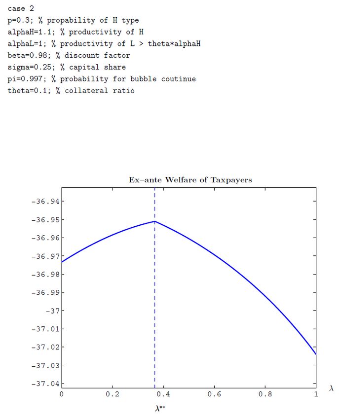
Here let us show you numerical examples. Figure are numerical exam-
ples showing the relationship between ex-ante welfare for tax payers and :
Parameter values are shown in Table. The di¤erence between each of four
cases lies in the bursting probability of bubbles. The lower is, the higher
the bursting probability is.
21
Smaller means that the share of the wage income over aggregate output is larger
relative to the share of the total bailout money. As a result, the marginal cost by expansion
of the bailout becomes small and the marginal bene…t is more likely to dominate the
marginal cost. This is the reason the slope of V0ex ante evaluated at = 0 is positive if
is small enough.
25These Figures show very interesting features. In the case of riskier bub-
bles, ex-ante welfare is maximized below the value of which maximizes
ex-ante e¢ ciency in production, i.e., < . This suggests that if the gov-
ernment wants to maximize ex-ante welfare for tax payers, it has to give up
some e¢ ciency in production, allowing L-entreprenurs to produce. Intuition
is the following. In the case of riskier bubbles, L-entrepreneurs do not want
to invest a lot of their savings in risky bubble assets. They end up with in-
vesting more part of their savings in their own L-projects for risk-hedge. In
this situation, in order to crowd L-projects out completely, the government
needs to rescue a greater fraction of entrepreneurs (remember that is an
decreasing function of :), which directly increases bailout money. Moreover,
when entrepreneurs anticipate that a greater fraction of them is rescued, this
generates a large increase in bubble prices and creates large size bubbles.
These two e¤ects produce large costs for tax payers, requiring large amounts
of public funds when bubbles collapse. Thus ex-ante welfare starts decreasing
when > : In 2 [0; ) ; ex-ante welfare increases because the welfare-
enhancing e¤ect dominates the welfare-reducing one. On the other hand,
in the case of safer bubbles, ex-ante e¢ ciency in production is achieved by
rescuing a smaller fraction of entrepreneurs. This means that total bailout
money does not become too large, requiring small amount of public funds
during the bubbles’collapsing. The welfare-enhancing e¤ect dominates the
welfare-reducing one until = : Thus ex-ante welfare is maximized at
= :
Our results show that the government faces dilemma. When …nancial
markets are imperfect, enough resources cannot be transferred to the produc-
tive sector. The presence of asset bubbles and government bailout improve
this situation, helping to smooth resource allocations from L-entrepreneurs
to H-entrepreneurs. However, if the government tries to improve resource al-
locations by expanding bailout, on one hand, production e¢ ciency enhances,
which improves tax payers’welfare. But on the other hand, bailout money
increases, which lowers their welfare. In the case of riskier bubbles, the latter
e¤ect becomes too large. Thus, from tax payers’point of view, the govern-
ment cannot but give up some e¢ ciency in resource allocations.
Moreover, our results also have interesting implications for boom-bust
cycles. Figure compares boom-bust cycles in three cases, = 0; = ;
and = . We consider the case where < : The charts in the
Figure show that boom-bust cycles become milder, because production is
not e¢ cient. This suggests that in order to maximize ex-ante welfare for tax
26payers, the government needs to mitigate boom-bust cycles.
27References
[1] Aoki, Kosuke, Gianluca Benigno, and Nobuhiro Kiyotaki. 2009. “Adjust-
ing to Capital Account Liberalization,”London School of Economics.
[2] Aoki, Kosuke, and Kalin Nikolov. 2011. “Bubbles, Banks and Financial
Stability,”The University of Tokyo.
[3] Bernanke, Ben, and Mark Gertler. 1989. “Agency Costs, Net Worth,
and Business Fluctuations,”American Economic Review, 79(1): 14–31.
[4] Bernanke, Ben, Mark Gerlter, and Simon Gilchrist. 1999. “The Financial
Accelerator in a Quantitative Business Cycle Framework,” in J. Taylor
and M. Woodford eds, the Handbook of Macroeconomics, 1341-1393.
Amsterdam: North-Holland.
[5] Brunnermeier, Markus, and Yuliy Sannikov. 2011. “The I Theory of
Money,”mimeo, Princeton University.
[6] Caballero, Ricardo, and Arvind Krishnamurthy. 2006. “Bubbles and
Capital Flow Volatility: Causes and Risk Management,” Journal of
Monetary Economics, 53(1): 35-53.
[7] Chari, Varadarajan V., and Patrick J. Kehoe. 2010. “Bailouts, Time-
Inconsistency, and Optimal Regulation,” mimeo Minneapolis Fed and
Princeton.
[8] Diamond, Douglas, and Raghuram Rajan. 2011. “Illiquid Banks, Finan-
cial Stability, and Interest Rate Policy,”Chicago University.
[9] Farhi, Emmanuel, and Jean Tirole. 2009a. “Bubbly Liquidity,” forth-
coming in Review of Economic Studies.
[10] Farhi, Emmanuel, and Jean Tirole. 2009b. “Leverage and the Central
Banker’s Put,” American Economic Review Papers and Proceedings,
99(2): 589-593.
[11] Farhi, Emmanuel, and Jean Tirole. 2011. “Collective Moral Hazard,
Maturity Mismatch and Systemic Bailouts,” forthcoming in American
Economic Review.
28[12] Gertler, Mark, Nobuhiro Kiyotaki, and Albert Queralto. 2011. “Finan-
cial Crises, Bank Risk Exposure and Government Financial Policy,”
forthcoming in Journal of Monetary Economics.
[13] Gali, Jordi, 2011. “Monetary Policy and Rational Asset Price Bubbles,”
Universitat Pompeu Fabra.
[14] Grossman, Gene, and Noriyuki Yanagawa. 1993. “Asset Bubbles and
Endogenous growth,”Journal of Monetary Economics, 31(1): 3-19.
[15] Hart, Oliver, and John Moore. 1994. “A Theory of Debt Based on the In-
alienability of Human Capital,”Quarterly Journal of Economics, 109(4):
841–879.
[16] Hellwig, Christian, and Guido Lorenzoni. 2009. “Bubbles and Self-
Enforcing Debt,”Econometrica, 77(4): 1137-1164.
[17] Hirano, Tomohiro, and Noriyuki Yanagawa. 2010a. “Asset Bubbles, En-
dogenous Growth, and Financial Frictions,” Working Paper, CARF-F-
223, The University of Tokyo.
[18] Hirano, Tomohiro, and Noriyuki Yanagawa. 2010b. “Financial Insti-
tution, Asset Bubbles and Economic Performance,” Working Paper,
CARF-F-234, The University of Tokyo.
[19] Holmstrom, Bengt, and Jean Tirole. 1998. “Private and Public Supply
of Liquidity,”Journal of Political Economy, 106(1): 1-40.
[20] Kamihigashi, Takashi, 2009. “Asset Bubbles in a Small Open Economy,”
Kobe University.
[21] Kiyotaki, Nobuhiro, 1998. “Credit and Business Cycles,”The Japanese
Economic Review, 49(1): 18–35.
[22] Kiyotaki, Nobuhiro, and John Moore. 1997. “Credit Cycles,”Journal of
Political Economy, 105(2): 211-248.
[23] Kiyotaki, Nobuhiro, and John Moore. 2008. “Liquidity, Business Cycles
and Monetary Policy,”Princeton University.
[24] Kocherlakota, R. Narayana. 1992. “Bubbles and Constraints on Debt
Accumulation,”Journal of Economic Theory, 57(1): 245-256.
29[25] Kocherlakota, R. Narayana. 2009. “Bursting Bubbles: Consequences
and Cures,”University of Minnesota.
[26] Korinek, Anton. 2011. “Systemic Risk-Taking: Ampli…cation E¤ects,
Externalities, and Regulatory Responses,” mimeo University of Mary-
land.
[27] Lorenzoni, Guido. 2008. “Ine¢ cient Credit Booms,”Review of Economic
Studies, 75(3): 809-833.
[28] Martin, Alberto, and Jaume Ventura. 2011a. “Theoretical Notes on Bub-
bles and the Current Crisis,”Forthcoming in IMF Economic Review.
[29] Martin, Alberto, and Jaume Ventura. 2011b. “Economic Growth with
Bubbles,”Forthcoming in American Economic Review.
[30] Matsuyama, Kiminori. 2007. “Credit Traps and Credit Cycles,”Ameri-
can Economic Review, 97(1): 503-516.
[31] Matsuyama, Kiminori. 2008. “Aggregate Implications of Credit Market
Imperfections,” in D. Acemoglu, K. Rogo¤, and M. Woodford, eds.,
NBER Macroeconomics Annual 2007, 1-60. University of Chicago Press.
[32] Miao, Jianjun, and Pengfei Wang. 2011. “Bubbles and Credit Con-
straints,”mimeo, Boston University.
[33] Nikolov, Kalin. 2010. “Is Private Leverage Excessive?,”MPRA Paper.
[34] Sakuragawa, Masaya. 2010. “Bubble Cycles,”mimeo, Keio University.
[35] Santos, S. Manuel, and Michael Woodford. 1997. “Rational Asset Pricing
Bubbles,”Econometrica, 65(1): 19-58.
[36] Tirole, Jean. 1982. “On the Possibility of Speculation under Rational
Expectations,”Econometrica, 50(5): 1163-1182.
[37] Tirole, Jean. 1985. “Asset Bubbles and Overlapping Generations,”
Econometrica, 53(6): 1499-1528.
[38] Tirole, Jean. 2005. The Theory of Corporate Finance. Princeton, New
Jersey: Princeton University Press.
30[39] Weil, Philippe. 1987. “Con…dence and the Real Value of Money,”Quar-
terly Journal of Economics, 102(1): 1-22.
[40] Woodford, Michael. 1990. “Public Debt as Private Liquidity,”American
Economic Review, 80(2): 382-388.
31Givenθ andαH,
Bubble Regions
0 π1(λ) π
π1 is a decreasing function ofλ.
When bailout is expected, even riskier bubbles can occur.
WhenαH is relatively low
Kt+1
booms bubbly dynamics
bust
dynamics in
bubbleless economy
Kt
Dynamic Effect of Stochastic Bubbles on the saddle path
32Yt (1≦t≦s) At date s, bubbles collapse.
J H1 < J H < J H2
λ↑→ZtL↓, ZtH↑ λ↑→ZtH↓
ZL=0
0 λ=λ* λ=1 λ
Value of λwhere ex-ante efficiency is maximized.
Yt (1≦t≦s) At date s, bubbles collapse.
J H ³ J H2
λ↑→ZtH↓
λ=0 λ=1 λ
Value of λwhere ex-ante efficiency is maximized.
33Pt ZHt
birth burst
t=0 t=s t t=0 t=s t
Yt Ct
t=0 t=s t t=0 t=s t
λ=λ* λ=0 bubbleless steady-state
34dt wt
birth burst
t=0 t=s t t=0 t=s t
s Lt
d t ¯ P t X/KAt : size of bubbles
s Lt ¯ Z Lt /KAt : share of L-projects
t=0 t=s t
λ=λ* λ=0 bubbleless steady-state
Kt+1
bubbly dynamics
when λ=λ*
bubbly dynamics
whenλ=0
dynamics in
bubbleless economy
Kt
Anticipated Bailout and Bubbly Dynamics
35Pt ZHt
birth burst
t=0 t=s t t=0 t=s t
Yt Ct
t=0 t=s t t=0 t=s t
λ=λ* λ=0 λ** bubbleless steady-state
36dt wt
birth burst
t=0 t=s t t=0 t=s t
s Lt
d t ¯ P t X/KAt : size of bubbles
s Lt ¯ Z Lt /KAt : share of L-projects
t=0 t=s t
λ=λ* λ=0 λ** bubbleless steady-state
37Ex-ante Welfare for Tax Payers
J H ³ J H2
λ**=0 λ=1 λ
Value of λwhere ex-ante welfare for tax payers is maximized.
3839
40
41
42
You can also read