The rate of return on capital in Germany - an empirical study Thomas Weiß - an empirical study ...
←
→
Page content transcription
If your browser does not render page correctly, please read the page content below
The rate of return on capital in Germany - an empirical study

                                                Thomas Weiß

        19th FMM Conference, “The Spectre of Stagnation? Europe in the World Economy”

                                    Berlin Steglitz, 22-24 October 2015

1) Stagnation and the rate of return on capital/rate of profit

Stagnation is defined in English Wikipedia (2015/8/28) as “a prolonged period of slow
economic growth (traditionally measured in terms of the GDP growth), usually accompanied
by high unemployment.” This must not necessarily imply low rates of return for capital (or low
rates of profit, which is in the following used synonymously), if, for instance, profits were used
for consumption and not for investment. On the other hand, scenarios might be possible
where high rates of growth go together with low rates of return, if, for example, growth is
financed not out of profits, but out of savings of workers or out of taxes. Generally however, it
is expected that rates of return/rates of profit are closely connected with GDP growth rates
(cf. Arnold 1997, p. 6f.). This again, however, leaves open the question whether stagnation
can be a peaceful final stage of economic development or whether a “Marxian apocalypse”
destroys any stable socioeconomic or political equilibrium (cf. Piketty 2014, p.9).1

In any case, classical economists expected a long term decline of rates of profit. For Adam
Smith competition would drive down profits. David Ricardo following Malthus thought that a
growing population needs the use of less fertile lands. The amount of labour necessary to
produce food would rise, therefore the value of food, which necessitates a rise in the wage of
workers.2 Rising wages cause a fall in the rate of profit in industry (“Ricardian apocalypse”,
Piketty p. 6).

Karl Marx with his law of the tendency of the rate of profit to fall assumed that “living labour”,
more precisely the surplus value creating part of wage labour, would be replaced by
“constant capital” (especially “fixed capital”, that is machines and equipment).3 The rate of
growth of productive wage labour would decline and, by this, value creation would fall behind
the value of accumulated capital.4 In the words of Piketty again this “principle of infinite
accumulation … kill[s] … the engine of accumulation”, leads to violent conflict among
capitalists or unites workers in revolt (cf. Piketty 2014, p.9).

In Marx’s scenario the “organic composition of capital”, that is the capital-output ratio, rises,
or its reciprocal value, capital productivity, declines. Crucial in this respect is the ratio of fixed
capital to value added. A “rationality trap” could consist in the fact that it makes sense for
individual firms to invest more in fixed capital, and less in employment, to increase labour

1
  For a possible repetition of a 30s style world crisis cf. Homburg (2015).
2
  As Marx (Speech by Marx to the First International Working Men's Association, June 1865) explained it (without
mentioning Ricardo) in „Wage, price, and profit“: “If, for example, in the progress of population it should become
necessary to cultivate less fertile soils, the same amount of produce would be only attainable by a greater amount
of labour spent, and the value of agricultural produce would consequently rise.”
(https://www.marxists.org/archive/marx/works/1865/value-price-profit/) Cf. also Callinicos 2014, p. 258ff.
3
  Cf. Schmalwasser, Schidlowski (2006a): „Die Produktion wird immer kapitalintensiver, weil zunehmend Arbeit
durch Kapital ersetzt wird. Also wächst der Kapitalstock schneller als die Produktion.“ (Production becomes more
capital intensive as capital progressively substitutes labour. Therefore the capital stock grows faster than the
output.)
4
  Marx reasons on the basis of the labour theory of value. For more details of this theory see Fröhlich (2010a and
b), Sinn (1975). For Marx’s law itself see Callinicos (2014), p. 261ff.
                                                                                                                 1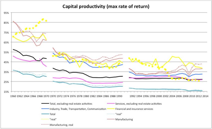
productivity and thus competitiveness. For the economy as a whole, however, this could
result in lower growth of employment and of consumption. The microeconomic individual
effort of companies to increase production per worker is met by the macroeconomic
constraint of total demand, with Marx measured in labour values. Rising wages per worker
can raise the demand for consumption in physical terms but not in value.5 As a result the rate
of profit declines.

2) Political implications

Crucially in this scenario a fall in the rate of profit, if any, is not due to higher wages, but to a
fall in capital productivity (a rise in the capital-output-ratio). Beginning with Marx6 this
scenario is traditionally used to assert the transience of capitalism. Capitalism is bound to
make room for a new “mode of production”. On the other hand, some economists close to
the trade unions see this scenario as a left version of supply side economics.7 If the law were
true, this would support the policy propositions of neoliberal economists. “Austerity” is then a
justified political “countervailing factor” (Marx) to dampen the fall of the rate of profit and to
maintain the stability of the economy. Indeed, with the German so-called RWI-DIW-debate of
the 1980s the conservative mainstream met Marxists to claim exactly the same, namely an
economy threatened by a falling capital productivity, whereas on the other side institutes
closer to positions of the trade unions challenged this and ascertained the healthy and stable
profitability of German firms (cf. Funke 1987, p. 190f.). The following treatise wants to shed
new light on the issues involved to underpin empirically further debates and discussions. In
addition to the rate of return on capital other magnitudes relevant in this context are
presented, namely the capital productivity and the rate of accumulation of capital.8

3) Concepts and data of the study

In the following the rate of return on fixed capital and the capital productivity are defined as
net operating surplus and gross value added, each in current prices, in relation to gross fixed
assets at replacement costs.9 Consumption of fixed capital is measured in current prices.10

5
  Marx is close to acknowledge that a balanced growth as assumed by modern steady-state growth models is
possible but dismisses that as a pure “abstract” coincidence (cf. Marx, Capital, vol. III, XIII.39).
6
  Karl Marx in Das Kapital Volume III, XV, 4: “Those economists who, like Ricardo, regard the capitalist mode of
production as absolute, feel nevertheless, that this mode of production creates its own limits, and therefore they
attribute this limit, not to production, but to nature (in their theory of rent). But the main point in their horror over
the falling rate of profit is the feeling, that capitalist production meets in the development of productive forces a
barrier, which has nothing to do with the production of wealth as such; and this peculiar barrier testifies to the
finiteness and the historical, merely transitory character of capitalist production. It demonstrates that this is not an
absolute mode for the production of wealth, but rather comes in conflict with the further development of wealth at
a certain stage.” (http://www.econlib.org/library/YPDBooks/Marx/mrxCpC15.html#Part III, Chapter 15)
7
  Mattfeldt (2006), p. 11: „Insofern schafft unsere Feststellung, dass die Profitrate tendenziell nicht fällt, sondern
eher steigt, wieder Raum für eine alternative Wirtschaftspolitik, die nicht den von den Entdeckern des
Profitratenfallgesetzes vorgeprägten angebotsorientierten Weg gehen muss.“ (In so far our finding that there is no
tendency for the rate of profit to fall, but rather to rise, makes room again for an alternative economic policy that
must not follow the road - preordained by our discoverers of the law of the rate of profit to fall - of supply side
economics.)
8
  For earlier studies for Germany see for example Hoffmann (1965), Priewe (1988), Lindlar (1998), Bontrup
(2000), Weiß (2015), Krüger (2015).
9
  A usual business economics definition is: Rate of return of capital employed = Earning before interest and tax
(EBIT) / Capital employed
10
   For authors who use the net capital stock instead to compute the rate of return, see for example Hoffmann
(1965, p. 98ff., p. 216), Duménil, Lévy (1993, p. 354) or Lindlar (1997, p. 358). This results in different levels but
not in different tendencies of development.
                                                                                                                       2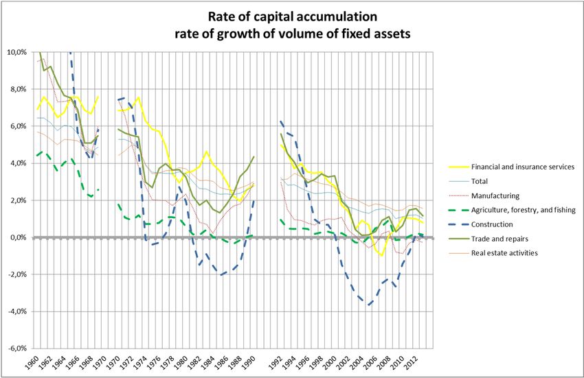
Table 1 presents the net operating surplus and gross fixed assets as items of the national
accounts:

Table 1: From “output” via “value added” to “net operating surplus”

              English terms                                      German terms
I. Production account:                         I. Produktionskonto
Output                                         Produktionswert
- Intermediate consumption                     - Vorleistungen
= Gross value added -> capital                 = Bruttowertschöpfung -> Kapitalproduktivität
productivity
- Consumption of fixed capital                 - Abschreibungen
= Net value added                              = Nettowertschöpfung
II. 1.1 Generation of income                   II. 1.1 Einkommensentstehungskonto
= Net value added (+other subsidies            = Nettowertschöpfung (+Sonstige Subventionen
on production                                  - Sonstige Produktionsabgaben)
-other taxes on production)
- Compensation of employees                    - Arbeitnehmerentgelt
= Net operating surplus / Net mixed            =
income (net = after deduction of               Nettobetriebsüberschuss/Selbständigeneinkommen
consumption of fixed income) -> rate of        -> Rentabilität
return, rate of profit
Source: Statistisches Bundesamt (May 2015)

Table 2: Items of income and capital in the national accounts

                                               consumption of fixed capital

   gross value added                                     compensation of employees

                             net value added

                                                    net operating surplus / mixed income

                                                   gross fixed assets

         capital
                                                       inventories

                                                          cash

At the moment the stock of inventories is not published in the national accounts, they are not
part of the European System of Accounts (ESA 2010). Data of, for instance, the 1980s for

                                                                                               3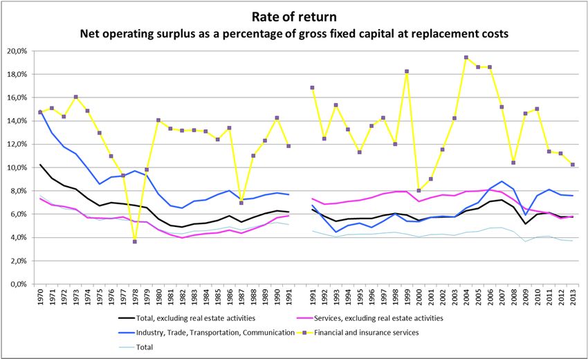
the old Federal Republic of Germany show, that inventories in comparison to fixed assets are
small (5% to 10%) but not negligibly small.

Fixed capital assets

There are several concepts to measure the capital stock. Gross fixed assets are recorded by
the Federal Statistical Office at current market prices of new fixed assets of a corresponding
quality. Net fixed assets are the fixed assets evaluated at current market value, or
alternatively as their original value minus consumption of fixed investment since the date of
the original investment (Schmalwasser, Schidlowski 2006b, p. 4). Schmalwasser and
Schidlowksi (p. 4) suggest that gross fixed assets as a measure of how much capital is in
use in production are the suitable value for measuring capital productivity. It is also suitable
as denominator in ratios describing the rate of return on capital, because assets have to be
replaced in total at their replacement costs and the income of the firm must be computed in
such a way as to prepare for that replacement.

Table 3: Possible concepts of “fixed capital” (with respect to computing the rate of
return)

                                       Net capital stock                      Gross capital stock
Historical prices at time of           Hoffmann (1965, p. 99,
purchase                               215f., 242)
Replacement costs                      Hoffmann, p. 246, Funke                Weiß 2015
                                       1996
Constant prices11                      Hoffmann, p. 244; Lindlar
                                       (1997, p. 358)

Relevant for the question whether the gross or the net approach should be used with fixed
assets with statistics of the total economy is, that investments in equipment become part of
the stock of equipment as part of fixed capital only after delivery to the buyer (an aeroplane is
part of fixed assets after delivery to the airline. Before, it is part of inventories). Capital
consumption (depreciation) begins after delivery. Building investments, however, become
part of fixed assets with the work in progress. For an autobahn, for instance, capital
consumption begins already when this road is still under construction.12

A more fundamental problem for the determination of the rate of return is, that, as often in
economics, it is not the present or past values, that matter, but the expected values, which,
however, cannot be observed. For the capitalist firm it is not about replacement of past
investments, but about staying competitive. This can mean the purchase of more expensive,
but efficient and competitive equipment. In this view, it is not about depreciation of past
investments, but about accumulating funds to be able to buy in the future the equipment
necessary to stay competitive. That the equipment which provides a higher productivity of
labour, might become more expensive, is a possible rationale for Marx’s law of the tendency
of the rate of profit to fall.

4) Results

11
   The Federal Statistical Office of Germany has abandoned to publish data for the capital stock at historical
prices “for capacity reasons” (Schmalwasser, Schidlowski 2006b, p. 4).
12
   For the precise definitions of and possible differences between “capital stock” and “fixed assets”, “investment”
and “fixed capital formation”, “depreciation” and “consumption of fixed capital” see Schmalwasser, Schidlowski
2006a or 2006b.
                                                                                                                      4
A long term view
Data as published by Thomas Piketty (2014) allow a longer term description of the
development of capital productivity and of the rate of return on capital. For Germany Piketty
uses data from Hoffmann (1965). Hoffmann presents data on capital income, net national
income and on the net capital stock at replacement costs and at constant prices. Using these
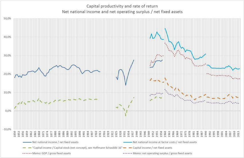
data of Hoffmann/Piketty in Figure 1 capital productivity and the rate of return on fixed
capital, defined as the net national income or the net operating surplus in relation to net fixed
assets, are presented.
Capital productivity and the rate of return on capital were quite stable in Germany till the First
World War. They resumed their path at a lower level after the war, then saw a short-lived
recovery during the “Roaring Twenties”, only to collapse soon during the World Depression.
But a quick and strong recovery followed which lasted till the beginning of the Second World
War.
In the light of the then available data of the Federal Statistical Office, the Second World War
lifted these rates, due to the destruction of fixed assets. But the rates, beginning in the 60s,
started to fall, in this post-war era of reconstruction, till 1982. From then onwards, a
stabilisation can be observed.13
The data of the Federal Statistical Office and of Hoffmann overlap for the 1950s, but they do
not fit well together. The Hoffmann data have net fixed assets about 70% larger than the
values provided by later publications of the Federal Statistical Office for 1950. Hoffmann
seems to have underestimated the destruction caused by the war. Net national income is
about the same than that of the Federal Statistical Office. The difference in capital
productivity between the two sources stems from the difference with respect to net fixed
assets.
13
Duménil and Lévy (1993, p. 248, p. 354ff.) show also a strong recovery of these rates for the United States, due
to the diminution of capital during and the recovery of income after the Great Depression.
5Figure 1: A long-term view
Source: Thomas Piketty: http://piketty.pse.ens.fr/en/capitalisback, “Germany.xls”, Hoffmann (1965, especially
“Schaubild 16” with “Rendite”, “Tabelle 40”, capital stock in current prices, total capital stock minus public
buildings and structures, “Tabelle 122”, “Volkseinkommen” as net national income, labour and capital income),
Statistisches Bundesamt (“VGR 1950 bis 1970”; August 2006; 7. September 2015), computations by author.
Although net national income of Hoffmann does not differ much from later values published
by the Federal Statistical Office, his capital income in the 50s is only about 60% of the
Federal Statistical Office value (Hoffmann’s wage share is larger). Together with the
mentioned higher estimation for net fixed assets this results in comparison with the data of
the Federal Statistical Office in a significantly lower rate of return, which is with Hoffmann
roughly at the level of the pre-war years.
From the 1960s onward
The Federal Statistical Office provides data beginning around 1950. More detailed data are
available from the 1960s onwards. Major statistical breaks are territorial changes with
respect to the Saarland and West-Berlin, finally German unification. Major methodical
changes were the change from the “all phases sales tax” to the Value added tax in 1968. In
2014 the Federal Statistical Office introduced the new European System of Accounts 2010
(ESA 2010). Data were revised back to 1991. 1991 marks a double structural break, one due
to German unification, and the other due to data revisions beginning with 1991.
In Figure 2 value added as a percentage of gross fixed assets at replacement costs is
shown. For comparison and as a check of the results for some branches the “‘real’
(physicalist) rate” (Kliman 2012, p. 119) of capital productivity is also shown by the dotted
lines. These rates, however, tell roughly the same story. The conspicuous divergence
between the capital productivities as measured in current prices or in constant prices in the
61950s with “Financial and Insurance Services” stems from a divergence between the
development of fixed assets whether measured at replacement costs or at constant prices.
Figure 2: Capital productivity 1960s onwards
Sources: Statistisches Bundesamt (“VGR 1950 bis 1970”; August 2006; 7. September 2015), computations by
author.
The rate of return on fixed capital follows more or less the development of the capital
productivity, at lower levels. A decisive turn-around happened in 1982. Since then not only
capital productivity, but also the rate of return was rather stable. The downward tendency of
the former years did not continue. There was even some improvement for the rate of return,
which indicates the long-term fall in the wage share. But in this age of neoliberalism, which
followed the paradigm of Keynesianism, there was no return to the high rates of the post-war
era.
7Figure 3: The rate of return
Source: Statistisches Bundesamt (August 2006, 7. September 2015), computations by author.
Rate of capital accumulation
The falling rate of profit leads to a falling rate of capital accumulation, measured as rate of
growth of fixed capital assets, measured in constant prices (Figure 4a) or as net capital
formation in relation to gross fixed assets at replacement costs (Figure 4b)14. Capital
accumulation follows the ups and downs of the business cycle. After 2000 “manufacturing”
saw longer spells of a shrinking capital stock. This reduction of the capital stock is an
important countervailing factor. It curbs the rise of the capital-output ratio and can mitigate a
fall of the rate of profit. The flip side of this is, of course, a lower demand for investment.
14
For a more sophisticated study on the rate of capital accumulation see Knetsch (2012).
8Figure 4a: The rate of capital accumulation
Source: Statistisches Bundesamt (“VGR 1950 bis 1970”; August 2006; 7. September 2015), computations by
author.
Figure 4b: The rate of capital accumulation
Source: Statistisches Bundesamt (August 2006, 7. September 2015), computations by author.
95) Results based on data provided by the Deutsche Bundesbank
Balance sheets of enterprises, as published by the Deutsche Bundesbank, comprise for
capital all non-financial assets, as shown in Table 4b, and all financial assets. These items
are evaluated at market prices. Thus, fixed assets are presented according to the net
approach.
Table 4a: Income statement
Income statement
Sales
+ Changes in finished goods
= Gross revenue
+ Interest and similar income
+ Other income
= Total income
- Cost of materials
- Personnel expenses
- Depreciation
- Interest and similar expenses
- Operating taxes
- Other expenses
= Annual result before taxes on income
- Taxes on income
= Annual result
Source: Deutsche Bundesbank
Table 4b: Balance sheet
Assets Capital
Non-financial assets Equity
Fixed assets (market value) Liabilities
Inventories Provisions
Financial assets Deferred income
Cash
Receivables
Securities
Other long-term equity
investments
Prepaid expenses
Balance sheet total
Source: Deutsche Bundesbank
Computed on this basis, the rate of return, that is “annual result and interest and similar
expenses” (Table 4a) in relation to the balance sheet total (Table 4b) followed a longer and
smoother downward path and stabilised in the 90s (Figure 5). An analysis of the balance
sheets provides some interesting additional information. Financial assets as part of total
assets rose steadily from about 40% in 1970 to around 60% now (see Annex TABLE 2 and
3). There is a dependence of non-financial corporations on the financial sector, but not on the
capital side of the balance, but on the assets side. The bail-out of the banks was in fact a
bail-out of German corporations. Interest expenses followed the ups and downs of the rate of
interest, which is a lagging indicator of the business cycle.
10Otherwise these statistics confirm the findings based on the national accounts. Personnel
expenses (wage costs) declined in the long run as a percentage of gross revenue, so did
operating taxes (Annex TABLE 1). Cash holdings as a percentage of the balance sheet total
increased, reflecting mounting risks (Annex TABLE 2). “Capital productivity” declined in the
sense that gross revenue as a percentage of the balance sheet total is now lower than it was
in the 1970s (Annex TABLE 3).
Figure 5: Results based on balance sheet data
Source: Deutsche Bundesbank, Special Statistical Publication 5 and 6, Excel-file 1970-1996, computations by
author.
6) Summary, interpretation, conclusions, further questions
At first sight, looking at Figure 1 it could seem as if in Germany the rates of profit and capital
productivity were quite stable since Prussian times. Major disturbances resulted from the
Great Depression in the years 1929 and after, and due to the Second World War. Capital
destruction during this war seems to have raised the ratios of profit and capital productivity.
The post-war period can be interpreted as a return to normalcy, rates declined and are now
roughly at their levels of the 19th century.
But this would be too sanguine a view. True, 1982 was something of a turning point.15 From
then onwards some stabilisation of the capital productivity and the rate of return can be
observed. In this sense, 1982 marked a paradigm shift from Keynesianism to Neoliberalism.
Whereas Keynesian policies were not able to stabilise the capitalist economy, neoliberal
ones seem to have achieved that. Especially important, the theoretical maximum rate of
profit, capital productivity, was also stabilised from 1982 onwards. There was, however, no
turn-around back to former levels of high rates of growth. Rates of profit or capital
15
For the US see Kliman (2012), p. 111; Henwood (2003), p. 204.
11productivities of the 1960s are beyond reach. Rates of profit benefited also from declining
labour shares. A deeper world wide division of labour with longer value chains and just-in-
time production might have caused the stabilisation of capital productivity.
To evaluate the results one has to look behind the surface of this stability since the 80s. It is
true, that this study does not provide indication for a hypertrophy of financial markets. The
trends for “financial and insurance services” are not that different from those of the other
branches of the economy. Rates of return were higher there, but also more volatile. Balance
sheet data show that indeed enterprises have now invested 60% of their capital in financial
assets, whereas in 1970 it was 40%. But for an exporting nation like Germany with a positive
investment position it might seem natural that its economic subjects, including the
enterprises, accumulate financial assets with respect to the rest of the world. Financial
investments abroad, which at the same time financed German exports, substituted domestic
investments. But this highlights also a possible vulnerability of the German economy with
respect to developments of the economy of the world at large.16
With respect to financial markets a further question is whether the development of German
stock prices, the stability of which till 1982 was followed by a lift-off, responds in any way to
the fall of the rate of profit till 1982 followed by a stabilisation.
Finally, the role of Keynesianism in a world of profit rates under pressure is to be debated. It
could still be argued that a concerted effort to raise public demand increases capacity
utilisation and capital productivity against the trend. If these fiscal stimuli are financed out of
taxes on profits, this must not diminish profits after taxes, if profits before taxes rise enough
due to the stimuli.
Left critiques use to complain about public-private partnerships as another form of
privatisations. But PPP implies by its very logic, even if everything is supposed to be in the
interest of private enterprise, more state intervention in investment decisions of enterprises,
as some conservative commentators correctly acknowledge. So we are not so far away from
Keynes’s famous suggestion of a “somewhat comprehensive socialisation of investment”
(Keynes 1936, chapter 24). If in the light of persistent low rates of profit more and more state
intervention becomes necessary, then that intervention can also be summoned for a social
policy beyond a mere stabilisation of the economy.
Literature
Arnold, L. (1997): Wachstumstheorie. München.
Bontrup, Heinz-J. (2000): Zur säkularen Entwicklung der Kapitalrentabilität. WSI-Mitteilungen
53 (11), S. 718-725
Callinicos, Alex (2015): Deciphering Capital - Marx’s capital and its destiny. London.
Deutsche Bundesbank (2006, 2015): Special Statistical Publication 5. Extrapolated results
from financial statements of German enterprises. Frankfurt.
16
For studies about possible financial losses in the wake of the financial crisis see Erik Klär, Fabian Lindner,
Kenan Sehovic (2013): Investition in die Zukunft? Zur Entwicklung des deutschen Auslandsvermögens.
Wirtschaftsdienst 93/3. European Commission, Macroeconomic Imbalances Germany 2014, European Economy
Occasional Papers 174. Deutsche Bundesbank Monthly Report May 2014, p. 48ff.
12Deutsche Bundesbank (2004, 2005, 2007, 2008): Special Statistical Publication 6. Ratios
from financial statements of German enterprises. Frankfurt.
Duménil, Gérard and Dominique Lévy (1993): The Economics of the Profit Rate -
Competition, Crises and Historical Tendencies in Capitalism. Aldershot.
Fröhlich, Nils (2010a): Die Überprüfung klassischer Preistheorien mithilfe von Input-Output-
Tabellen, in: Wirtschaft und Statistik 2010 (5), S. 503-508.
Fröhlich, Nils (2010b): Labour values, prices of production and the missing equalization of
profit rates: Evidence from the German economy (https://www.tu-
chemnitz.de/wirtschaft/vwl2/downloads/paper/froehlich/deviation.pdf)
Funke, M. (1987): Einflüsse auf die Entwicklung der Kapitalrentabilität im verarbeitenden
Gewerbe in der Bundesrepublik Deutschland, in: Jahrbuch für Sozialwissenschaft, 38 (2), S.
188-209
Hoffmann, Walther (1965): Das Wachstum der deutschen Wirtschaft seit der Mitte des 19.
Jahrhunderts. Berlin, Heidelberg, New York.
Henwood, Doug (2003): After the New Economy. New York.
Homburg, Stefan (2015): What caused the Great Recession? Review of Economics, vol. 66
(2015), issue 1.
Keynes, John Maynard (1936): The General Theory of Employment, Interest and Money.
(available online: http://synagonism.net/book/economy/keynes.1936.general-
theory.html#idChap24SectIIPara4)
Kliman, Andrew (2012): The Failure of Capitalist Production - Underlying Causes of the
Great Recession. London.
Knetsch, Thomas A. (2012): A user cost approach to capital measurement in aggregate
production functions. Discussion Paper Deutsche Bundesbank No 01/2012
Krüger, Stephan (2015): Entwicklung des deutschen Kapitalismus 1950-2013 -
Beschäftigung, Zyklus, Mehrwert, Profitrate, Kredit, Weltmarkt. Hamburg.
Lindlar, Ludger (1997): Das mißverstandene Wirtschaftswunder - Westdeutschland und die
westeuropäische Nacahkriegsprosperität. Tübingen.
Mattfeldt, Harald (2006): Zur Methode der Profitratenbestimmung, Anmerkungen zur Empirie
der ‘Säkularen Entwicklung der Kapitalrentabilität’. Discussion Paper No. 01,
Profitratenanalysegruppe am Zentrum für Ökonomische und Soziologische Studien
(ZOESS), Universität Hamburg.
Piketty, Thomas (2014): Capital in the Twenty-First Century. Translated by Arthur
Goldhammer. Cambridge, MA, London.
Priewe, Jan (1988): Krisenzyklen und Stagnationstendenzen in der Bundesrepublik
Deutschland – Die krisentheoretische Debatte. Köln
13Schmalwasser, Oda; Michael Schidlowski (2006a): Kapitalstockrechnung in Deutschland.
Wirtschaft und Statistik 11/2006.
Schmalwasser, Oda; Michael Schidlowski (2006b): Measuring Capital Stock in Germany,
Slightly abridged version of a paper published in the journal Wirtschaft und Statistik 11/2006
Sinn, Hans-Werner (1975): Das Marxsche Gesetz des tendenziellen Falls der Profitrate.
Zeitschrift für die gesamte Staatswissenschaft 131, S. 646-696. [downloadable]
Statistisches Bundesamt (August 2006): Fachserie 18 Reihe S. 29. Volkswirtschaftliche
Gesamtrechnungen, Inlandsproduktsberechnung, Revidierte Jahresergebnisse, 1970 bis
1991. Wiesbaden.
Statistisches Bundesamt (May 2015): National Accounts, sector accounts, Annual results
1991 onwards. Wiesbaden.
Statistisches Bundesamt (September 2015): Fachserie 18 Reihe 1.4. Volkswirtschaftliche
Gesamtrechnungen, Inlandsproduktsberechnung, Detaillierte Jahresergebnisse, 2014.
Wiesbaden. [contains data from 1991 onwards]
Weiß, Thomas (2015): Sachkapitalrendite im historischen Vergleich - Deutschland im
Abwärtstrend? WSI Mitteilungen 4/2015
More on sources:
1950s:
Statistisches Bundesamt (Juni 1992): Volkswirtschaftliche Gesamtrechnungen, Fachserie 18,
Reihe S. 17 Vermögensrechnung, 1950 bis 1991.
Figure 1:
a) Net capital stock:
Hoffmann (1965), capital stock, net: Tabelle 40. Der Kapitalstock nach Wirtschaftsbereichen
in laufenden Preisen 1850-1959 (Mrd. Mark), Net capital stock = „insgesamt“ - „öffentliche
Gebäude“ - “öffentlicher Tiefbau”, capital income: (“Kapitaleinkommen”) Tabelle 122. Die
Verteilung des Nettosozialprodukts zu Faktorkosten in laufenden Preisen 1850-1959 (Mill.
Mark), Spalte 13. “Nettoinlandsprodukt” (net domestic income) Spalte 15.
Capital stock: 1950-1990: Reproduzierbares Sachvermögen am Jahresanfang, Mill. DM,
netto, ohne öffentlichen Tiefbau.
Nettoanlagevermögen, Alle Wirtschaftsbereiche 1991-2011, Statistisches Bundesamt,
Fachserie 18 Reihe 1.4, Volkswirtschaftliche Gesamtrechnungen,
Inlandsproduktsberechnung, Detaillierte Jahresergebnisse, 2013, Erscheinungsfolge:
jährlich, Erschienen am 05. März 2014
b) Net national income
Statistisches Bundesamt: Volkswirtschaftliche Gesamtrechnungen, Bruttoinlandsprodukt,
Bruttonationaleinkommen, Volkseinkommen, Lange Reihen ab 1925, 2014, Erschienen am
25.08.2015 Stand: August 2015. “Volkseinkommen” (net national income at factor costs)
14Nettoanlagevermögen, alle Wirtschaftsbereiche 1960-1998: Statistisches Bundesamt,
Volkswirtschaftliche Gesamtrechnung, Fachserie 18, Reihe 1.3, 1997, Hauptbericht.
Erschienen im Oktober 1998.
c) Gross capital stock:
Capital stock: 1950-1990: Reproduzierbares Sachvermögen am Jahresanfang, Mill. DM,
brutto, ohne öffentlichen Tiefbau.
Gross fixed assets: 1991-2014: Statistisches Bundesamt, Fachserie 18 Reihe 1.4,
Volkswirtschaftliche Gesamtrechnungen, Inlandsproduktsberechnung, Detaillierte
Jahresergebnisse, 2014, Erscheinungsfolge: jährlich. Erschienen am 09. März 2015
Gross fixed assets, Bruttoanlagevermögen, alle Wirtschaftsbereiche 1960-1998:
Statistisches Bundesamt, Volkswirtschaftliche Gesamtrechnung, Fachserie 18, Reihe 1.3,
1997, Hauptbericht. Erschienen im Oktober 1998.
15Annex
TABLE 1
Income statement of enterprises
1971 1980 1990 1998 2004 2006 2007 2009 2013
% of gross revenue
Interest income 1971-1998 0,5 0,5 0,6 0,6
1997-2009 0,5 0,4 0,4 0,5 0,4
2006-2013 0,5 0,6 0,4 0,3
Other income 1971-1998 2,5 2,7 3,3 4,6
1997-2009 4,0 4,0 4,0 4,3 4,5
2006-2013 4,3 4,8 4,7 4,2
Cost of materials 1971-1998 59,1 60,9 60,3 59,4
1997-2009 58,0 59,6 61,4 61,6 60,0
2006-2013 61,1 60,9 61,1 63,6
Personnel
expenses 1971-1998 19,4 18,9 18,3 17,4
1997-2009 18,5 17,3 15,7 15,4 16,6
2006-2013 15,4 15,0 15,6 14,8
Depreciation 1971-1998 3,8 3,3 3,7 3,4
1997-2009 3,4 2,9 2,6 2,5 2,7
2006-2013 3,2 3,1 3,3 2,6
Interest expenses 1971-1998 1,6 1,7 1,5 1,2
1997-2009 1,2 1,0 0,9 1,0 1,0
2006-2013 1,1 1,2 1,1 1,0
Operating taxes 1971-1998 2,9 2,6 2,8 3,2
1997-2009 1,6 1,6 1,5 1,4 1,5
2006-2013 1,4 1,2 1,4 1,1
Other expenses 1971-1998 10,0 10,4 11,4 13,4
1997-2009 13,5 13,9 13,5 13,2 14,6
2006-2013 13,6 13,4 14,3 13,0
Total expenses 1971-1998 96,9 97,9 97,9 98,1
1997-2009 96,3 96,3 95,6 95,1 96,4
2006-2013 95,8 95,0 96,8 96,2
1971-1998 3,1 2,1 2,1 1,9
Annual result 1997-2009 2,7 2,8 3,5 3,9 2,8
2006-2013 3,3 4,0 2,4 3,1
Annual result 1971-1998 - - 3,4 3,2
before taxes on
income 1997-2009 3,7 3,7 4,4 4,9 3,6
2006-2013 4,2 5,0 3,2 3,8
Source: Deutsche Bundesbank, computations by author.
16TABLE 2
Balance sheet, Assets
1971 1980 1990 1998 2004 2006 2007 2009 2013
% of balance sheet total
Intangible fixed
assets 1971-1998 -
1997-2009 1,5 2,1 2,0 2,0 1,9
2006-2013 2,5 2,4 2,3 2,0
Tangible fixed
assets 1971-1998 36,3 29,9 27,5 24,3
1997-2009 23,6 21,8 20,6 19,6 20,5
2006-2013 25,9 25,0 25,3 23,4
Inventories 1971-1998 27,9 31,2 26,0 23,3
1997-2009 23,2 19,4 18,4 19,1 18,7
2006-2013 15,0 16,0 15,6 16,4
Non-financial
assets 1971-1998 64,1 61,1 53,5 47,6
1997-2009 48,3 43,4 41,1 40,6 41,2
2006-2013 43,3 43,3 43,1 41,7
Cash 1971-1998 4,1 4,2 5,2 4,6
1997-2009 5,7 7,0 7,0 6,9 8,1
2006-2013 6,3 6,1 7,1 7,0
Receivables 1971-1999 25,5 27,6 30,9 32,1
1997-2010 33,0 33,3 35,4 35,9 33,3
2006-2013 32,5 32,5 31,7 33,1
Securities 1971-1998 0,6 1,4 2,2 3,4
1997-2009 2,5 2,7 2,8 2,4 2,6
2006-2013 3,0 2,7 2,9 2,1
Other long term 1971-1998 5,2 5,4 7,7 11,9
equity
investments 1997-2009 10,0 13,1 13,1 13,7 14,2
2006-2013 14,3 14,8 14,6 15,5
Financial assets 1971-1998 35,4 38,6 46,1 52,0
1997-2009 51,2 56,1 58,4 58,9 58,2
2006-2013 56,2 56,2 56,3 57,8
Prepaid expenses 1971-1998 0,4 0,4 0,4 0,4
1997-2009 0,5 0,5 0,5 0,5 0,5
2006-2013 0,5 0,5 0,6 0,5
Source: Deutsche Bundesbank, computations by author.
17TABLE 3
Balance sheet, Capital
1971 1980 1990 1998 2004 2006 2007 2009 2013
% of balance sheet total
Equity 1971-1998 25,3 19,7 18,2 18,7
1997-2009 17,5 22,8 24,3 24,2 25,2
2006-2013 24,3 25,1 25,7 28,1
Short term 1971-1998 43,2 46,7 45,5 44,5
Liabilities 1997-2009 45,9 43,8 43,5 44,2 42,5
2006-2013 40,1 40,9 39,1 40,3
Long term 1971-1998 20,8 18,7 15,6 14,8
Liabilities 1997-2009 17,5 13,5 12,4 11,4 13,1
2006-2013 15,7 14,7 16,0 14,7
Provisions 1971-1998 10,3 14,5 20,4 21,7
1997-2009 18,7 19,4 19,3 18,7 18,7
2006-2013 18,9 18,4 18,3 16,0
Deferred income 1971-1998 0,5 0,4 0,3 0,4
1997-2009 0,3 0,4 0,4 0,4 0,5
2006-2013 1,0 0,9 0,9 0,8
Liabilities and 1971-1998 74,2 80,0 81,5 80,9
Provisions 1997-2009 82,5 77,2 75,7 74,7 74,8
2006-2013 75,7 74,9 74,3 71,9
Gross revenue 1971-1998 166,9 185,8 179,2 173,5
1997-2009 188,5 184,7 190,3 186,4 170,3
2006-2013 165,4 162,3 151,4 159,0
Source: Deutsche Bundesbank, computations by author.
18You can also read