"Australia's Country Towns 2050: What will a Climate Adapted Settlement Pattern look like?" - Professor Andrew Beer Centre for Housing, Urban and ...
←
→
Page content transcription
If your browser does not render page correctly, please read the page content below
“Australia’s Country Towns 2050:
    What will a Climate Adapted
   Settlement Pattern look like?”

             Professor Andrew Beer
Centre for Housing, Urban and Regional Planning
                  March 2012
Introduction
Composite Index of Vulnerability for UCLs in
Rural and Regional Australia
Aim: Increase understanding of how climate
change might affect rural and regional areas in
a differentiated way
– Objectives: Categorise Localities based on
Vulnerability Index
– Identify measures for local adaptation
• Beta version is tentative and simplifiedRationale
• Regional climate change has and is occurring
• 0.7oC warming since the early 1950s which has seen the
following trends:
more rain in north-western Australia
rain in southern an eastern Australia
Increased number of heatwaves
Less frosts
Longer and more intensive droughts (IPCC 2007)
• Impacts are being experienced in rural and regional
Australia such as:
Reduced water availability for both irrigated and rain fed
agriculture.
Increased vulnerability to extreme eventsVulnerability Index The IPCC (2007) state vulnerability is the degree to which: • a system is susceptible to, and • unable to cope with, • adverse effects of climate change, including climate variability and extremes. (IPCC 2007) Therefore vulnerability is a function of: • Exposure • Sensitivity • Adaptive Capacity
Vulnerability Index
Preparation of composite index was made via the following
  steps:
1. Conceptualize what makes UCLs more or less vulnerable
   and identify proxies covering key dimensions of climate
   change vulnerability
2. Select and collect statistical data to represent different
   vulnerability aspects/proxies (Approx 1550 UCLs in Index
   to date)
3. Interpret aspects and describe the aspects qualitatively,
   to determine direction of each factor (whether it
   increases or decreases vulnerability)
4. Normalise values for each proxy
5. Create index and rank each UCL
Data Sources
Main data Sources:
• OzClim
• ABS
• GISCA
In process/further investigations:
• ABARE
• DEEWR
• RPdata
Vulnerability Index
Index created using equal weights and simple average of
    all the normalised scores for each component (sub
    indices)of vulnerability using the following formula:
                   VI = (A + S + E)/3

Normalisation of indicators (min-max transformation
based on functional relationship):
   Method 1. Yij = ( X ij – Min X ij ) / ( Max X ij – Min X ij )
   Method 2. Yij = ( Max X ij – X ij ) / ( Max X ij – Min X ij )
Choice of indicators
Indicator/data Functional Rationale Normalisation
relationship method used
Exposure Percentage Change in Mean The higher the projected change the
Surface Temperature (%) , in more vulnerable is the UCL
AUSTRALIA for the year 2050,
1
Annual1
Percentage Change in Total The higher the projected change the
Rainfall (%) , in AUSTRALIA for more vulnerable is the UCL 1
the year 2050, Annual1
Sensitivity % Employed in Ag related The higher the proportion of people
Industries employed in Ag related industries the 1
more vulnerable is the UCL
Remoteness The more remote the UCL is the more
1
vulnerable it is
Adaptive % of total employed persons by The higher the proportion of people in
capacity Highest Year of School workforce completing year 12 the less 2
Completed vulnerable is the UCL
% of employed persons by age The higher the proportion of people in
by level of highest educational workforce with Tertiary education or
attainment; postgraduate (1); equivalent the less vulnerable is the UCL 2
grad diploma (2); and Bachelor
Degree (3).
Population number (size) The higher the total population the
2
less vulnerable is the UCL
% Population with internet The higher the proportion of people
access connected to the internet the less 2
vulnerable the UCL is
1. Model: CSIRO-Mk3.5. Emission Scenario: SRES marker scenario A1B, Global Warming
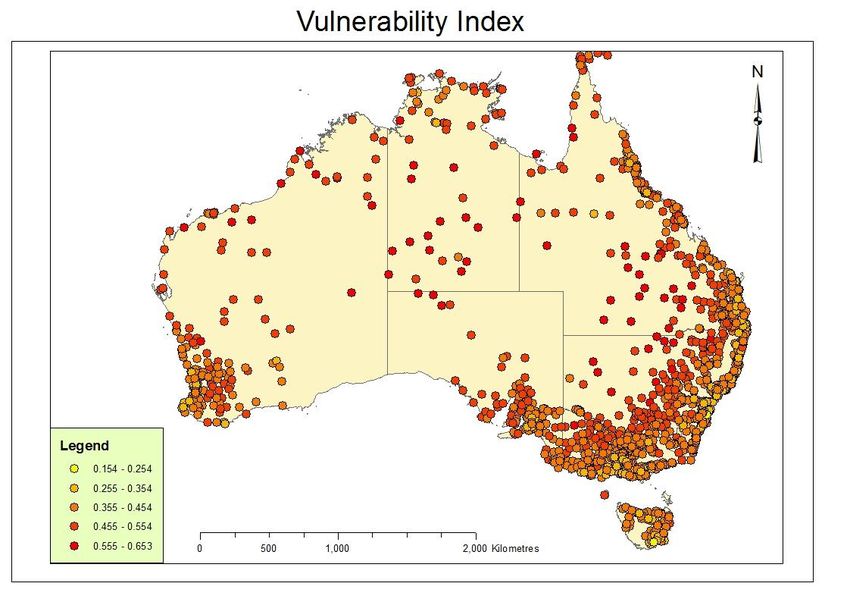
Rate: moderateMost Vulnerable
Vulnerability
UCL STATE PCODE Score Rank
Marble Bar (L) WA 6760 0.653 1
Tottenham (L) NSW 2873 0.644 2
Alpha (L) Qld 4724 0.635 3
Goodooga (L) NSW 2831 0.628 4
Quilpie (L) Qld 4480 0.617 5
Willowra (L) NT 0872 0.612 6
Cunnamulla Qld 4490 0.612 7
White Cliffs (L) NSW 2836 0.610 8
Ampilatwatja (Aherrenge) (L) NT 0872 0.609 9
Kaltukatjara (Docker River) (L) NT 0852 0.608 10
Ali Curung (L) NT 0862 0.605 11
Augathella (L) Qld 4477 0.602 12
Titjikala (L) NT 0872 0.601 13
Brewarrina NSW 2839 0.594 14
Elliott (L) NT 0862 0.593 15
Boulia (L) Qld 4829 0.593 16
Dirranbandi (L) Qld 4486 0.593 17
Ernabella (L) SA 0872 0.591 18
Thargomindah (L) Qld 4492 0.591 19
Looma (L) WA 6728 0.590 20Least Vulnerable
Vulnerability
UCL STATE PCODE Score Rank
Fern Tree (L) Tas 7054 0.154 1
Newcastle NSW 2300 0.221 2
Howden (L) Tas 7054 0.221 3
Woodbridge (L) Tas 7162 0.231 4
Crafers-Bridgewater SA 5154 0.236 5
Mount Nebo (L) Qld 4520 0.246 6
Central Coast NSW 2250 0.249 7
Stanwell Park NSW 2508 0.250 8
Wollongong NSW 2500 0.254 9
Summertown (L) SA 5141 0.254 10
Gundaroo (L) NSW 2620 0.254 11
Lauderdale Tas 7021 0.256 12
Kenthurst (L) NSW 2156 0.257 13
Geelong Vic 3220 0.261 14
Wooroowoolgan (L) NSW 2470 0.266 15
Dilston (L) Tas 7252 0.270 16
Otford (L) NSW 2508 0.271 17
Sunshine Coast Qld 4567 0.271 18
Talbot Islands (L) Qld 4875 0.274 19
Mount Glorious (L) Qld 4520 0.274 20Indigenous
• Many of the most vulnerable communities
appear to be the remote Indigenous
communities
– Low levels of education attainment
– Low levels of employment
– Some reliance on agricultural/pastoral
employment opportunities
– Small sizeMurray Darling Basin
• Includes both high risk and low risk centres
– Eg Albury Wodonga low risk, Darlington Point
higher risk
– More inland centres at greater risk
– No allowance for flows or rates of return on
irrigated investmentsSome limitations… • Composition of the index constrained by available sources of information preventing more coverage of variables and use of better proxies • Weighting of the various components is problematic – Field work will illuminate local factors that may affect weighting • Static Analysis – No time series data used for adaptive capacity and sensitivity
Preliminary Findings / conclusions
• Possible to map and assess vulnerability using
  a composite index
• Human factors create a somewhat unexpected
  pattern
  – Eg the robust circumstances of the coastal
    communities
  – Education, employment, industry structure are
    critical
• To be refined and weighted
References IPCC 2007 Fourth Assessment Report: Climate Change (AR4)
You can also read