Capybara Hélio Wang - Mar 09, 2020 - Capybara's documentation!
←
→
Page content transcription
If your browser does not render page correctly, please read the page content below

Capybara

 Hélio Wang

   Mar 09, 2020

Documentation

1   Installation                                                                                                                                                                                              3
    1.1 Download . . . . . . . . . . . . . . . . . . . . . . . . . . . . . . . . . . . . . . . . . . . . . . . . .                                                                                            3
    1.2 Build . . . . . . . . . . . . . . . . . . . . . . . . . . . . . . . . . . . . . . . . . . . . . . . . . . .                                                                                           3

2   Optimal enumeration                                                                                                                                                                                       5
    2.1 Definitions of tasks .   .   .   .   .   .   .   .   .   .   .   .   .   .   .   .   .   .   .   .   .   .   .   .   .   .   .   .   .   .   .   .   .   .   .   .   .   .   .   .   .   .   .   .    5
    2.2 Loading an input file    .   .   .   .   .   .   .   .   .   .   .   .   .   .   .   .   .   .   .   .   .   .   .   .   .   .   .   .   .   .   .   .   .   .   .   .   .   .   .   .   .   .   .    6
    2.3 Counting . . . . . .     .   .   .   .   .   .   .   .   .   .   .   .   .   .   .   .   .   .   .   .   .   .   .   .   .   .   .   .   .   .   .   .   .   .   .   .   .   .   .   .   .   .   .    8
    2.4 Listing . . . . . . .    .   .   .   .   .   .   .   .   .   .   .   .   .   .   .   .   .   .   .   .   .   .   .   .   .   .   .   .   .   .   .   .   .   .   .   .   .   .   .   .   .   .   .    9

3   Suboptimal enumeration                                                                                                                                                                                   11
    3.1 Basic usage . . . . . . . . . . . . . . . . . . . . . . . . . . . . . . . . . . . . . . . . . . . . . . . .                                                                                          11
    3.2 Example . . . . . . . . . . . . . . . . . . . . . . . . . . . . . . . . . . . . . . . . . . . . . . . . .                                                                                            11

4   Output visualization                                                                                                                                                                                     13
    4.1 Input format . . . . .       .   .   .   .   .   .   .   .   .   .   .   .   .   .   .   .   .   .   .   .   .   .   .   .   .   .   .   .   .   .   .   .   .   .   .   .   .   .   .   .   .   .   13
    4.2 Graphical elements . .       .   .   .   .   .   .   .   .   .   .   .   .   .   .   .   .   .   .   .   .   .   .   .   .   .   .   .   .   .   .   .   .   .   .   .   .   .   .   .   .   .   .   13
    4.3 Visualization methods        .   .   .   .   .   .   .   .   .   .   .   .   .   .   .   .   .   .   .   .   .   .   .   .   .   .   .   .   .   .   .   .   .   .   .   .   .   .   .   .   .   .   14
    4.4 Example . . . . . . .        .   .   .   .   .   .   .   .   .   .   .   .   .   .   .   .   .   .   .   .   .   .   .   .   .   .   .   .   .   .   .   .   .   .   .   .   .   .   .   .   .   .   14

5   Overview                                                                                                                                                                                                 17

6   Features                                                                                                                                                                                                 19

7   References                                                                                                                                                                                               21

                                                                                                                                                                                                              i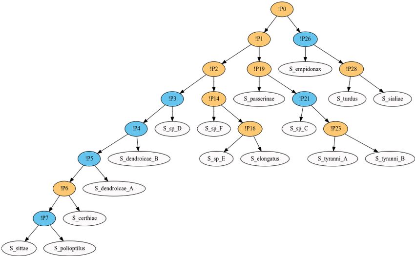
ii
Capybara

Capybara is a desktop application for solving the Phylogenetic tree reconciliation problem.
Keywords: Cophylogeny reconstruction, phylogenetic tree reconciliationm, enumeration.

Documentation                                                                                        1
Capybara

2          Documentation
CHAPTER     1

                                                                                               Installation

1.1 Download

Click here to get Capybara.
You can find the binary executables of Capybara for the following OS:
    • Microsoft Windows 10
    • macOs
    • Linux (Ubuntu, Fedora, Debian, Arch Linux, Manjaro, etc.)
Please note that no additional installation is required. Just unzip and double-click!
For some Linux versions: you might need to manually make the file executable in a terminal

chmod +x Capybara

1.2 Build

The source code is available at https://github.com/Helio-Wang/Capybara-app.
You may want to build Capybara from source if
    • You are not using one of the supported OS (Windows, macOS, major flavors of Linux), or
    • You have made some changes to the source code.
First, clone or create the project directory and

cd Capybara-app

Capybara includes a Pipfile specifying all requirements, generated by the virtual environment management tool
Pipenv. Install Pipenv if you don’t have it alreday:

                                                                                                           3
Capybara pip install pipenv Next, build the Pipenv virtual environment and install the requirements from Pipfile. Be sure that you already have Python 3.6 installed on your system. If you have multiple versions of Python, this command will automatically search for Python 3.6. pipenv install Then, you can execute the main script directly: pipenv run python main.py Alternatively, you can build and run the binary: pipenv install -d pipenv run python -OO -m PyInstaller main.py -F dist/./main For Windows 10 users: you also need to install pywin32-ctypes with pipenv install pywin32-ctypes. Note that, although Pipenv automatically scans for the targeted Python version (Python 3.6), this may not give the desired result if you have multiple implementations of Python (for instance, CPython 3.6.8 and PyPy 3.6.9). In this case, you can specify the path to the correct Python version, for example: pipenv --python /usr/bin/python3.6 4 Chapter 1. Installation
CHAPTER           2

                                                                                 Optimal enumeration

 Table of Contents

     • Optimal enumeration
          – Definitions of tasks

              * Task T1: All solutions
              * Task T2: Event vectors
              * Task T3: Event partitions
              * Task T4: Equivalence classes
          – Loading an input file
          – Counting

              * Basic usage
              * Example
          – Listing

              * Basic usage
              * Options for tasks T1 and T2
              * Options for tasks T3 and T4

2.1 Definitions of tasks

By choosing the option Standard counting and enumeration in Capybara, the user can either count or list one of the
following:

                                                                                                                5
Capybara
For a given input file and a given cost vector, let S be the set containing all reconciliations of minimum cost (cyclic or
acyclic).
2.1.1 Task T1: All solutions
Count: size of S.
Enumerate: the set S.
2.1.2 Task T2: Event vectors
Count: number of different event vectors in S.
Enumerate: all different event vectors in S.
The event vector of a reconciliation is a vector of four integers representing the number of occurrences of cospeciation,
duplication, host-switch, and loss events.
Two reconciliations have the same event vectors if the numbers of each event are the same.
2.1.3 Task T3: Event partitions
Count: number of different event partitions in S.
Enumerate: all different event partitions in S.
The event partition of a reconciliation is a partition of the internal nodes of the symbiont tree into three subsets:
cospeciation, duplicaiton, and host-switch nodes.
Two reconciliations have the same event partitions if, for each node in the symbiont tree, the assigned events (cospe-
ciation, duplication, host-switch) are the same, regardless of the hosts.
2.1.4 Task T4: Equivalence classes
Count: number of equivalence classes in S.
Enumerate: all equivalence classes in S.
Two reconciliations are considered equivalent if, for each node in the symbiont tree, the assigned events (cospeciation,
duplication, host-switch) are the same, moreover, the assigned hosts are also the same except when the event is a host-
switch.
2.2 Loading an input file
The input format is the same as for . Here is an example input file. Note that the symbiont tree
can be also introduced in a block starting with BEGIN SYMBIONT instead of BEGIN PARASITE.
After loading a file with the Open button, the input file information is displayed, and the other buttons become avail-
able:
Cost vector
• Before clicking on the Count or Enumerate button, choose the desired cost vector.
6 Chapter 2. Optimal enumerationCapybara 2.2. Loading an input file 7
Capybara

    • All four numbers must be integers.
    • Floating point numbers will be rounded towards zero (3.6 becomes 3, -3.6 becomes -3).
    • Different cost vectors can be used, for example, across differents runs of the counting tasks, without needing to
      re-load the input file.

Tip:
    • The file openning and saving dialogs have their own application-wide favorites list. The user can add a folder to
      favorites using drag and drop to have quicker access in the futur.
    • Not sure what an option means? Most buttons and boxes have help messages (tooltip). These will appear when
      the mouse cursor moves over an item.

2.3 Counting

2.3.1 Basic usage

The user can check multiple boxes in Task then click on the Count button for the results to be printed directly in the
Output area.
It is possible to save the on-screen text output to a file using the Save button.

2.3.2 Example

Here is the output of all four counting tasks on the example input:

===============
Job started at 2019-09-20 15:24:52
Cost vector: (-1, 1, 1, 1)
------
Task 1: Counting the number of solutions (cyclic or acyclic)...
Total number of solutions = 18
------
Task 2: Counting the number of solutions grouped by event vectors...
1: [8, 1, 6, 2] of size 4
2: [9, 1, 5, 4] of size 2
3: [9, 0, 6, 4] of size 4
4: [8, 0, 7, 2] of size 8
Total number of event vectors = 4
Total number of solutions = 18
------
Task 3: Counting the number of event partitions...
Total number of event partitions = 4
------
Task 4: Counting the number of strong equivalence classes...
Total number of strong equivalence classes = 4
------
Optimal cost = 1.0
------
Job finished at 2019-09-20 15:24:52
                                                                                                   (continues on next page)

8                                                                                   Chapter 2. Optimal enumeration
Capybara
(continued from previous page)
Time elapsed: 0.71 s
===============
2.4 Listing
2.4.1 Basic usage
Use the Enumerate button for listing solutions to a file that can be used for analysis or visualization. Unlike the Count
button, it allows only one task box to be checked at a time.
After choosing the output file name, the user selects additional options, depending on the task. Once the additional
options are confirmed, the computation starts automatically, and a progress bar pops out. It is possible to stop the
computation at anytime by closing the progress bar (the program may freeze for a few seconds).
Note that the on-screen text output (human-readable trace of computational tasks) can still be saved using the Save
button.
2.4.2 Options for tasks T1 and T2
The output is in the same format as the output of . And just like in , the user can choose the maximum
number of solutions that she likes to generate.
For the task T1 (all optimal reconciliations) only, it is possible to keep only the acyclic reconciliations.
Here is an example of the on-screen output when this option is chosen, for another input file and cost vector
(0,1,1,1):
===============
Job started at 2019-09-20 19:40:04
Cost vector: (0, 1, 1, 1)
Task 1: Enumerate acyclic solutions...
------
Number of acyclic solutions = 144 out of 184
Optimal cost = 11.0
Output written to C:/Users/Public/Test/output.txt
------
Job finished at 2019-09-20 19:40:05
Time elapsed: 0.63 s
===============
2.4.3 Options for tasks T3 and T4
There are two output types:
Labels only
If the first output type “labels only” is chosen, the result will be compatible with the new visualization
tool Capybara Viewer.
Task T3: Each event partition is represented by the assignment, to each internal symbiont node, of one of
the three events.
2.4. Listing 9Capybara
Task T4: Each equivalence class is represented by the assignment, to each internal symbiont node, of one
of the three events, and the assignment of a host hame to each symbiont node with non-host-switch event.
Reconciliation
If the second output type “reconciliation” is chosen, the result will be compatible with the the original
viewer for .
Note that in this case, the output is only one reconciliation chosen arbitrarily among the potentially many
(cyclic or acyclic) reconciliations having the same event partition or belonging in the same equivalence
class.
10 Chapter 2. Optimal enumerationCHAPTER 3
Suboptimal enumeration
The input format is the same as for Optimal enumeration (see Loading an input file).
3.1 Basic usage
Consider all reconciliations of a given input ordered by cost in a list, then the K-best solutions is the first K element
of this list.
Note that the ordering between solutions having the same cost is arbitrary.
K-best solution enumeration allows to obtain sub-optimal solutions if the number K is fixed to be larger than the
number of optimal solutions.
3.2 Example
For this input file and cost vector (0,1,2,1), there are 40 solutions having the optimal cost 21 (none of which
is acyclic), and 396 solutions having the second-optimal cost 22 (146 are acyclic).
By fixing K = 100 (without filtering by cyclicity), the output will contain 100 solutions. The first 40 are the optimal
solutions, and the next 60 are chosen arbitrarily among the 396 second-optimal solutions.
The choice of these 60 solutions are arbitrary, meaning that if the user closes and restarts the program, the output may
be different in spite of using exactly the same input.
If the cyclicity filter is applied, the output will contain a certain number of acyclic solutions: it’s the number of acyclic
solutions among the 60 second-optimal solutions. This number varies each time the program restarts, and it might be
zero.
11Capybara 12 Chapter 3. Suboptimal enumeration
CHAPTER 4
Output visualization
For visualizating reconciliations (symbiont tree drawn on top of the host tree), use the original viewer for .
For visualizating event partitions or equivalence classes (colorings of the parasite tree with animation), use the new
animated web tool Capybara Viewer.
Next we present the usage of the new visualization tool.
4.1 Input format
The Capybara visualizer tool takes two input formats generated from the third tab Convert enumeration files for
visualization of the main Capybara tool:
• File input (DOT format) can be saved into the filesystem by clicking the Save button. This file needs to be
uploaded into Capybara viewer after selecting the first upload method.
• Plain text input can be copied into the user’s clipboard by clicing the Copy button. Then the clipboard content
can be pasted into Capybara viewer.
Note that the text area for copy-and-paste is hidden by default, and will only appear after the user selects the
second upload method Copy and paste text.
Note: When the Capybara app closes, the clipboard content will also be cleared. Therefore, if you choose the second
upload method, do not close the main app while using the viewer.
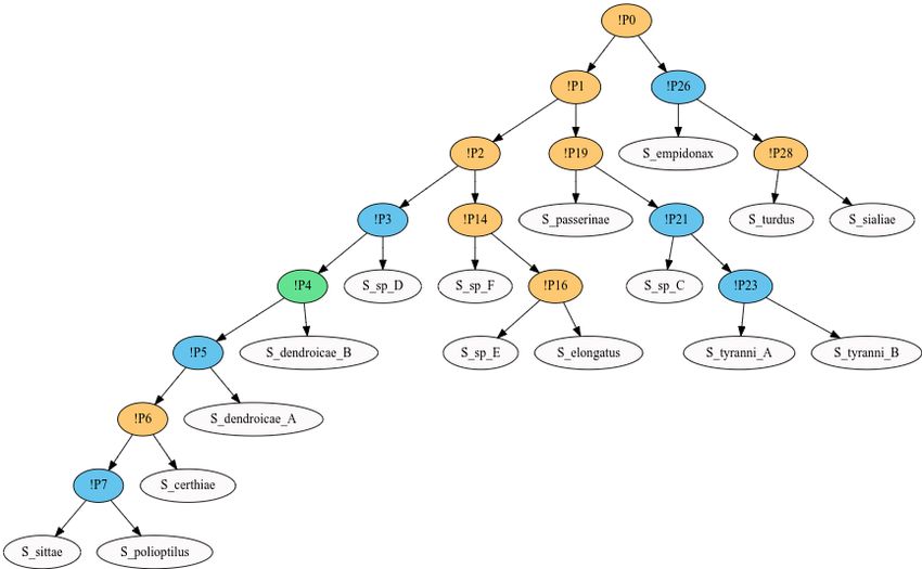
4.2 Graphical elements
One event partition or equivalence class will be drawn as a colored symbiont tree.
Texts The names of the nodes in the symbiont tree are shown.
13Capybara
Colors The internal nodes of the symbiont tree are colored according to the event. The correspondance between color
and event is shown in the legend on top of the graphic area.
Hover texts When the mouse hovers over a node, the corresponding host name, if known, is shown in small tag. This
applies to all leaf nodes of the symbiont tree, or, in an equivalence class, those internal nodes with non-host-
switch event.
4.3 Visualization methods
One frame of the animation corresponds to one event partition, or one equivalence class.
The user can:
• Either play the animation, i.e., a continous transition of images from one frame to another. The transition time
can be adjusted. This method is interesting because it can provide a quick global view on multiple solutions.
Combined with a screen-recording tool, it can also produce a video output.
• Or freeze the animation at one particular frame. This can be useful for checking the host names in equivalence
classes.
A single frame can be saved in a image file, either by using the save button on top of the legend, or by using the cell
menu (this menu appears when clicking the three small dots on the top left corner of the graphic area).
4.4 Example
There are 4 event partitions on this example input file and cost vector (-1,1,1,1). Thereofre, there are 4
frames in the animation.
Frame 1:
Frame 2:
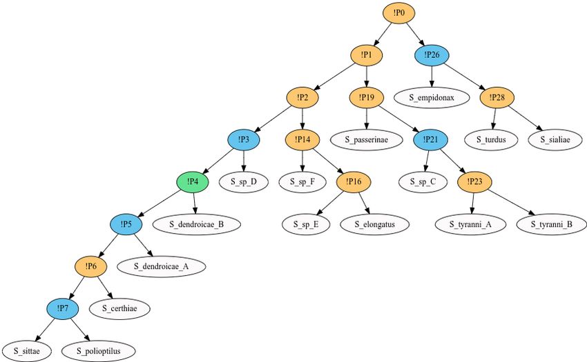
Frame 3:
Frame 4:
14 Chapter 4. Output visualizationCapybara 4.4. Example 15
Capybara

16         Chapter 4. Output visualization
CHAPTER           5

                                                                                                      Overview

Phylogenetic tree reconciliation is the method of choice in analyzing host-symbiont systems. Despite the many
reconciliation tools that have been proposed in the literature, two main issues remain unresolved:
    • listing suboptimal solutions (i.e., whose score is “close” to the optimal ones), and
    • listing only solutions that are biologically different “enough”.
The first issue arises because the optimal solutions are not always the ones biologically most significant; providing
many suboptimal solutions as alternatives for the optimal ones is thus very useful. The second one is related to the
difficulty to analyze an often huge number of optimal solutions.
Capybara addresses both of these problems in an efficient way. Furthermore, it includes a tool for visualizing the
solutions that significantly helps the user in the process of analyzing the results.

                                                                                                                  17
Capybara 18 Chapter 5. Overview
CHAPTER               6

                                                                                                                             Features

                                                                            1
Capybara has some features in common with its predecessor                     : counting the number of optimal reconcilia-
tions, listing optimal reconciliations to a file, keeping only the acyclic ones (the definition of cyclicity is taken from2 ).

 Wow! New features!

   1 Beatrice Donati, Christian Baudet, Blerina Sinaimeri, Pierluigi Crescenzi, and Marie-France Sagot. Eucalypt: efficient tree reconciliation

enumerator. Algorithms for Molecular Biology, 10(1):3, 2015. doi: 10.1186/s13015-014-0031-3.
   2 Maureen Stolzer, Han Lai, Minli Xu, Deepa Sathaye, Benjamin Vernot, and Dannie Durand. Inferring duplications, losses, transfers and

incomplete lineage sorting with nonbinary species trees. Bioinformatics, 28(18):i409–i415, 2012. doi: 10.1093/bioinformatics/bts386.

                                                                                                                                           19
Capybara
Capybara also has some exciting new features:
• Counting and enumeration of even vectors, event partitions, equivalence classes (see the Definitions of tasks in
Optimal enumeration)
• Enumeration of suboptimal reconciliations (see Suboptimal enumeration)
• Animated visualization of event partitions and equivalence classes (see Output visualization)
20 Chapter 6. FeaturesCHAPTER 7
References
21You can also read